2. The GP is kriging

The Gaussian process is not a rival to kriging, and learning it is not a change of field. It is a re-derivation of the kriging model from a Bayesian point of view. Every quantity a geostatistician already trusts (the weights, the estimation variance, the variogram) reappears here under another name, computed by the same linear algebra. What changes is what the pieces mean, and that change of reading is what the rest of the manual builds on. Once the variogram is a prior and the kriging system is a conditioning step, replacing the Gaussian assumption, stacking models or attaching a categorical variable all become natural moves rather than new theories.

Throughout the manual, lowercase letters are scalars (\(z\), \(r\)), bold lowercase letters are vectors (\(\mathbf{x}\), \(\mathbf{z}\)), and bold uppercase letters are matrices (\(\mathbf{K}\)). \(\mathcal{N}\) is the Gaussian distribution.

2.1 Simple kriging, restated

Take \(N\) samples \(z_1, \dots, z_N\) at locations \(\mathbf{x}_1, \dots, \mathbf{x}_N\), a known stationary mean \(m\), and a covariance function \(k(\mathbf{x}, \mathbf{x}')\) fitted to the data. Simple kriging estimates the value at a new location as a weighted average of the samples, with the weights \(\boldsymbol{\lambda}\) solving one linear system per target location:

\[ \left[\mathbf{K}_{NN} + \sigma_0^2 \mathbf{I}\right] \boldsymbol{\lambda} = \mathbf{k}_0, \]

where \(\mathbf{K}_{NN}\) holds the covariances between samples, \(\mathbf{k}_0\) the covariances between the samples and the target, and \(\sigma_0^2\) is the nugget. The estimate is \(\hat{z}_0 = m + \boldsymbol{\lambda}^T (\mathbf{z} - m)\), and the estimation variance follows from the same quantities.

Now the Bayesian derivation of the same numbers. Model the ground as a random function \(f(\mathbf{x})\) with a Gaussian process prior, meaning only this: any set of locations, read jointly, is multivariate Gaussian, with mean \(m\) and covariances given by \(k\). Model each sample as that function plus measurement noise, \(z_i = f(\mathbf{x}_i) + \epsilon_i\) with \(\epsilon_i \sim \mathcal{N}(0, \sigma_0^2)\). Conditioning the prior on the \(N\) observed values gives a posterior distribution at any set of new locations, and it is Gaussian with

\[ \boldsymbol{\mu}_G = \mathbf{K}_{GN} \left[\mathbf{K}_{NN} + \sigma_0^2 \mathbf{I}\right]^{-1} (\mathbf{z}_N - \mathbf{m}_N) + \mathbf{m}_G \]

\[ \boldsymbol{\Sigma}_G = \mathbf{K}_{GG} - \mathbf{K}_{GN} \left[\mathbf{K}_{NN} + \sigma_0^2 \mathbf{I}\right]^{-1} \mathbf{K}_{NG}. \]

The posterior mean is the simple kriging estimate, from the same system and the same weights, location by location, and the diagonal of the posterior covariance is the simple kriging variance. Nothing was gained yet, and nothing was lost. The GP at this point is kriging with its assumptions written out as a probability model instead of left implicit in the estimator.

Three readings change, though, and each buys something later:

The variogram is a prior. It states what the field is believed to do before the data speak, so fitting it becomes a statistical estimation problem with a likelihood rather than a curve-fitting exercise on the experimental variogram (§2.3).
The answer is a distribution. The kriging variance stops being an abstract “estimation variance” and becomes the width of an actual predictive distribution, something that can be simulated from, warped, and checked against held-out data (chapter 13).
The noise is a model component. The nugget \(\sigma_0^2\) sits in the likelihood, the measurement model, and not in the covariance of the ground. The posterior above filters it, so predictions are of \(f\), the ground, with the scatter of the assays averaged out. Kriging with measurement error makes the same move. Here it is the default, and chapter 4 builds a whole doctrine on the distinction.

In the code. geoml.models.GP is this model, closed form and single-variable, the legacy entry point kept for exactly this correspondence. Modern work goes through geoml.models.VGPNetwork (chapter 3), which contains the GP as its simplest case. The nugget is the noise parameter of geoml.likelihood.Gaussian, and the covariance function is assembled in §2.2’s box.

2.2 Covariance functions are variogram models

Under stationarity the two spellings carry the same information. With sill \(\sigma_1^2\),

\[ \gamma(h) = \sigma_0^2 + \sigma_1^2 - k(h) \quad (h > 0), \]

so the familiar variogram models are covariance functions read upside down. geoML writes them on a normalized distance \(d\), scaled so that the ranges parameter is the practical range, the distance where the structure has effectively vanished. That is how a fitted variogram is read in practice:

model	covariance	variogram behaviour
spherical	\(\sigma_1^2 (1 - 1.5d + 0.5d^3)\) for \(d \le 1\), else \(0\)	reaches the sill exactly at the range
exponential	\(\sigma_1^2 \exp(-3d)\)	95% of the sill at the range
Gaussian	\(\sigma_1^2 \exp(-3d^2)\)	parabolic at the origin: very smooth fields

The choice among them is the same judgement it always was. The behaviour at the origin is the model’s opinion about short-range continuity, and the Gaussian model’s extreme smoothness is as double-edged here as in kriging. Nested structures are sums of covariances, as before.

Anisotropy enters through the distance:

\[ d = \sqrt{(\mathbf{x} - \mathbf{x}')^T \mathbf{A}^T \mathbf{A} (\mathbf{x} - \mathbf{x}')}, \]

with \(\mathbf{A}\) encoding the search-ellipsoid geometry: ranges along principal directions, and the rotation placing them in space. In geoML the matrix is a spatial transform object handed to the covariance, which is a more consequential design than it looks. Transforms chain, so a fault, a projection or a learned deformation composes with the ellipsoid instead of requiring a new kernel. Chapters 3 and 5 use this freely.

In the code. geoml.kernels.Covariance(kernel=..., transform=...) assembles the pieces: kernels.Spherical(), kernels.Exponential(), kernels.Gaussian() for the function, and geoml.transform.Isotropic, Anisotropy2D, Anisotropy3D for the ellipsoid, with ChainedTransform to compose them. The ranges and angles are trainable parameters, which is the subject of the next section.

2.3 Fitting: maximum likelihood instead of the eye

The traditional workflow fits the variogram to the experimental one. That step is subjective, sensitive to binning and to the practitioner, and the experimental variogram’s pointwise behaviour is treacherous enough that the risks were documented long ago (Cressie, 1985). The probability-model reading replaces it: the variogram parameters (ranges, sill, nugget, anisotropy angles) are chosen to maximize the likelihood of the data under the model. Variogram modelling is GP training with a Gaussian likelihood, with one objective, no bins, gradients available, and every parameter including the rotation angles estimated jointly.

The price is printed on the same line. The likelihood involves \(\left[\mathbf{K}_{NN} + \sigma_0^2\mathbf{I}\right]^{-1}\) and its determinant, which cost \(\mathcal{O}(N^3)\): fine at hundreds of samples, heavy at ten thousand assays, impossible at a hundred thousand. Kriging’s classical answer is the search neighbourhood, solving small local systems and accepting the artefacts (discontinuous maps, negative weights, a variance that ignores most of the data). The variational answer keeps one global model and makes it sparse instead. That is chapter 3, and it is the reason this package exists.

2.4 Walker Lake, the short way

The bundled Walker Lake set runs the whole correspondence in a few lines. It holds 470 samples of the classic V variable, a second variable U, and the prediction grid. Printing the container’s tree is the habit worth forming: every variable, every column, and what is filled in so far.

import os

import geoml

os.makedirs("figures", exist_ok=True)
geoml.set_seed(1234)

walker, walker_grid = geoml.datasets.walker()
print(walker.tree())

PointData - 470 locations
|-- V                          ContinuousVariable
|   |-- measurements           float64
|   |-- latent_mean            empty
|   |-- latent_variance        empty
|   |-- prediction             empty
|   |-- dispersion             empty
|   `-- noise_variance         empty
`-- U                          ContinuousVariable
    |-- measurements           float64
    ...

The empty columns are the ones a prediction fills. Now look at the sampling:

figure = geoml.plots.Explorer(walker, continuous="V").scene(clip=[0, 0.99])
figure.savefig("figures/02-walker-samples.png", dpi=150)

The Walker Lake samples

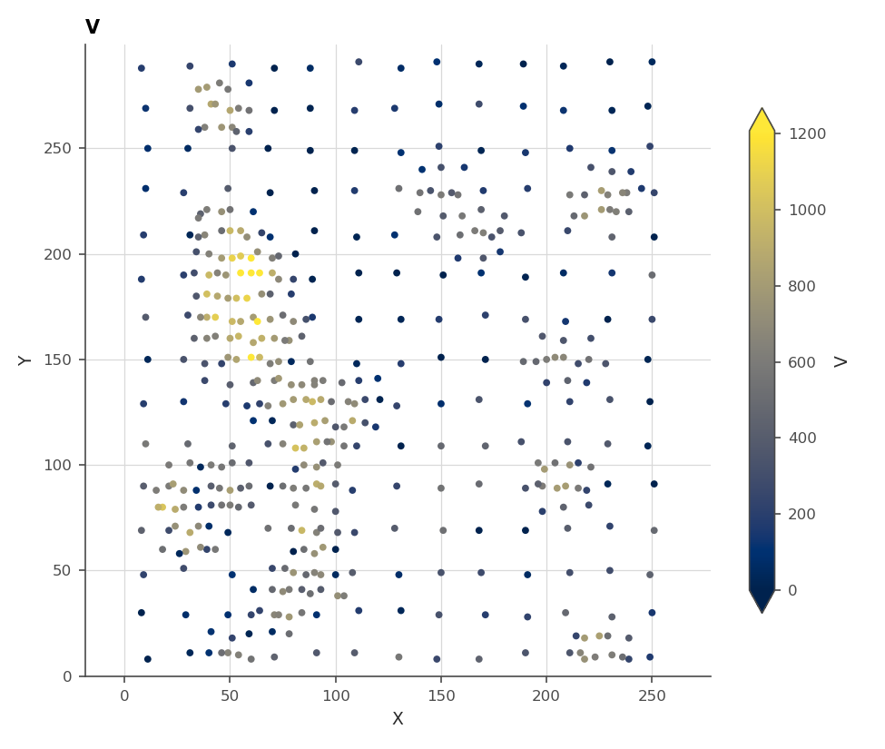
The sampling is already the story half told: dense lines and sparse gaps, so any validation that ignores the geometry will lie (chapter 13). The model is three objects. The ZScore warping standardizes the variable, which is all the plain model needs. Chapter 4 does far more with warpings.

covariance = geoml.kernels.Covariance(
    kernel=geoml.kernels.Spherical(),
    transform=geoml.transform.Isotropic(100.0))

model = geoml.models.GP(
    data=walker,
    variable="V",
    covariance=covariance,
    warping=geoml.warping.ZScore(1),
    options=geoml.models.GPOptions(verbose=False))

model.train(20)
print(model)

Training moved the range, sill and nugget to their maximum-likelihood values. No experimental variogram was drawn, and printing the model shows where the parameters landed, each with the bounds it was allowed to move in. This printout is the fitted variogram, and reading it is the same habit as reading a variogram model before kriging with it.

Prediction fills the grid with the posterior: the kriging estimate, and simulated realizations to cut intervals from.

import matplotlib.pyplot as plt

model.predict(walker_grid, n_sim=20)

walker_grid.get("V").reset_quantiles([0.05, 0.5, 0.95])
median = walker_grid.get("V/quantiles/0.5").as_image()
spread = walker_grid.get("V/quantiles/0.95").as_image() \
    - walker_grid.get("V/quantiles/0.05").as_image()

figure, axes = plt.subplots(1, 2, figsize=(9, 4.2), sharey=True)

for ax, image, title in zip(axes, [median, spread],
                            ["median", "0.05-0.95 spread"]):
    drawn = ax.imshow(image, origin="lower", cmap="cividis")
    figure.colorbar(drawn, ax=ax, shrink=0.8)
    ax.set_title(title)

figure.savefig("figures/02-walker-posterior.png", dpi=150,
               bbox_inches="tight")

The posterior: median and spread

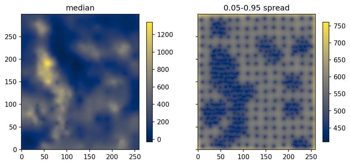
The median map is kriging’s map. The spread beside it is the part kriging computed and mostly discarded, widest exactly where the samples thin out. Whether that band can be believed is a question with machinery of its own, and chapter 13 is where it lives.

One property of this model deserves to be said out loud before anyone maps a grade with it:

import numpy as np

print("lowest simulated value:",
      round(float(np.min(walker_grid.values("V/quantiles/0.05"))), 1))

The number is negative. V is a positive variable, and nothing in the construction knows that. The latent field is Gaussian on the whole real line, and ZScore is a linear map, so the back-transform can return any value at all. Part of the predictive distribution therefore sits below zero wherever the model is unsure near low grades, which shows up in the lower quantiles first and in the mean of a skewed variable soon after. Kriging has the same defect and the same excuse. Chapter 4 fixes it properly, by putting a positivity warping between the field and the variable so that no realization can come back negative.

References

Chilès, J.-P., & Delfiner, P. (2012). Geostatistics: Modeling Spatial Uncertainty (2nd ed.). Wiley.

Cressie, N. (1985). Fitting variogram models by weighted least squares. Mathematical Geology, 17(5), 563–586.

Gonçalves, Í. G. et al. (2022). Learning spatial patterns with variational Gaussian processes: regression. Computers & Geosciences. https://doi.org/10.1016/j.cageo.2022.105056

Goovaerts, P. (1997). Geostatistics for Natural Resources Evaluation. Oxford University Press.

Rasmussen, C. E., & Williams, C. K. I. (2006). Gaussian Processes for Machine Learning. MIT Press.