11. Building and training

The theory chapters introduced every part. This one is the assembly manual: the order things must happen in, the knobs that matter, and the habits that make a model reproducible and recoverable. It is short on new ideas and long on the things that cost an afternoon when learned by surprise.

11.1 The order of construction

One rule outranks the others: seed first, then build. Parameter initialization draws from the package generator at construction, and a model’s options draw their own seed, for training’s Monte Carlo and the simulation stream, from the same generator when they are created. One call before any object exists makes the whole pipeline replayable.

import os

import geoml
import numpy as np

os.makedirs("figures", exist_ok=True)
geoml.set_seed(1234)          # before ANY model object is built

walker, walker_grid = geoml.datasets.walker()

Then the assembly, in the order the pieces depend on each other: inducing points, input node, GP node, warping, likelihood, model. Each one gets its own name, which costs a line and buys a network you can inspect a piece at a time.

experts = geoml.data.inducing.grid_experts(walker_grid, 10.0, block=8)

root = geoml.latent.BasicInput(
    experts,
    transform=geoml.transform.Isotropic(50))

gp = geoml.latent.BasicGP(
    root,
    size=1,
    kernel=geoml.kernels.Spherical())

warping = geoml.warping.ChainedWarping(
    geoml.warping.Scale(1),
    geoml.warping.Softplus(1),
    geoml.warping.ZScore(1),
    geoml.warping.Spline(1, knots_per_arm=4))

likelihood = geoml.likelihood.Gaussian(warping)

model = geoml.models.VGPNetwork(
    walker, "V",
    likelihood,
    gp,
    options=geoml.models.GPOptions(verbose=False))

print(model)

The repr is the model document: every node, every parameter, its bounds and whether it is fixed. Read it before training the way a variogram model is read before kriging. Most “why is it doing that” questions are answered in it.

Multi-variable models pass lists in matching order (["Elements", "Landuse"] with a likelihood each). Two places are worth a moment’s thought before training starts: the initial transform range, and the warping chain. Initialization is not fitting, but a range wrong by an order of magnitude starts the climb in a bad valley, and a chain without a positivity link will happily predict a negative grade (chapter 4).

11.2 Training, watching, adjusting

train_full(max_iter=...) for datasets that fit in a batch, train_svi past that (chapter 3). Adam runs underneath, and set_learning_rate is there for when the default is too bold for a delicate warping. Two habits matter.

model.train_full(max_iter=500)

figure = geoml.plots.Explorer(walker, continuous="V",
                              model=model).training_curve()
figure.savefig("figures/11-training-curve.png", dpi=150,
               bbox_inches="tight")

The ELBO and its running mean

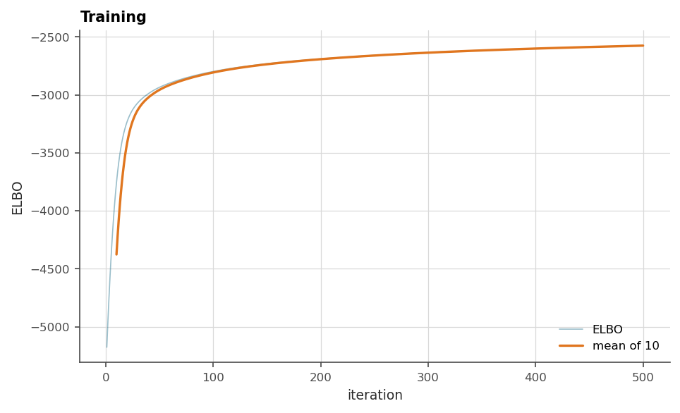
The first habit is to watch the running mean of the ELBO until it is flat. An unsettled fit gives seed-dependent answers, which is a reproducibility problem wearing a modelling problem’s clothes. The curve above is worth looking at closely: it rises steeply for the first fifty iterations and then keeps creeping for hundreds more. The steep part is the model finding the right scale, and the creep is the warping and the variational state settling against each other. Stopping at the elbow is the common mistake, and the flat tail is what the eye should be waiting for.

The second is to train in rounds. Another train_full call continues where the last one stopped, so predict, look and resume is the intended rhythm rather than a trick.

Two GPOptions are worth knowing beyond the defaults. jit_predict=True compiles prediction with XLA, measured at 3–5× on big grids, and is off by default because XLA refuses what it cannot compile instead of falling back. training_samples sets the Monte Carlo width of the ELBO estimate, and the default serves. Raise it only when the curve is too noisy to read.

11.3 Saving, loading, resuming

A trained model persists whole: structure, parameters, training data, even the seed it drew, so a reloaded model replays its simulations exactly.

import tempfile, os

os.makedirs("figures", exist_ok=True)
path = os.path.join(tempfile.mkdtemp(), "walker_model")
geoml.persistence.save_model(model, path)

restored = geoml.persistence.load_model(path)

fresh_grid = geoml.data.Grid2D(start=[1, 1], n=[50, 50], step=[5.2, 5.6])
restored.predict(fresh_grid, n_sim=8)

print("the reloaded model predicts:", "V" in fresh_grid.variables)
print("lowest value:",
      round(float(np.min(fresh_grid.values("V/prediction"))), 1))

The value is positive, as the Scale → Softplus → ZScore → Spline chain guarantees, and it is the same number the original model would have given.

The mechanism is worth understanding, because two workflows ride on it. Saving records the constructor calls that built every object, plus the parameter values they arrived at, and loading replays them. One consequence is that a class recorded in a save must keep its import path forever, which the package maintains shims for. The useful consequence is that load_model(path, data=another_container) rebuilds the same trained model around different data. That gives you the fitted structure as a starting point on a new drilling campaign, and it is the mechanism chapter 13’s cross-validation uses to build its fold models.

In the code. models.VGPNetwork, models.GPOptions, persistence.save_model and load_model, and stats/random.py for the one seed knob.

11. Building and training

11.1 The order of construction

11.2 Training, watching, adjusting

11.3 Saving, loading, resuming

Further reading