8. Change of support

Samples are points, and decisions are blocks. Between the two sits the oldest problem in mining geostatistics: a block’s grade distribution is narrower than a point’s, selectivity depends on support, and a resource computed at the wrong support is wrong in the direction that costs money. The classical toolkit corrects distributions after the fact, with affine and lognormal corrections or the discrete Gaussian model. This package takes the direct road instead and predicts the block as the average it is, by discretizing it, carrying every sub-block through the full model (warping, noise doctrine and all) and averaging in the variable’s own units. That is exact with respect to the model, needs no correction formula, and the same machinery then decides where the block model itself should be finer.

8.1 What a block prediction reports

A block fans out into sub-blocks on its way through the model, and comes back with the three variances of chapter 4 finally all on stage:

column	the question
prediction	the block’s value, the average of its interior
latent_variance	how sure the model is of that value
dispersion	how much the ground varies inside the block
noise_variance	how far an assay of it would scatter

dispersion is the volume–variance story told per block. It grows with block size and shrinks with continuity, and it is computed from the same field as the value, so the block and the statement about its interior never disagree.

Cut-offs make it operational. Declared once, on the data (variable.set_cutoffs([...])), they travel with the variable to every container predicted from it, and each block reports two different things about each cut-off:

• proportions is the share of the block above the cut-off, the recoverable fraction, the number a grade–tonnage curve integrates;

• divided is how often the realizations disagree about whether the cut-off crosses the block. This is the one that licenses refinement. A block whose realizations all agree, all ore or all waste, holds one answer however finely it is cut, while a block the cut-off genuinely crosses holds two, and only cutting can separate them.

8.2 The block model that refines itself

BlockSet3D is a variable-size block model with octree discipline. Every block’s origin and size are whole numbers of a base cell, split keeps the model tiling its box exactly, and discretization is both the sub-block fan-out and the refinement ratio, so (2, 2, 1) refines in plan and leaves the bench height alone. models.refine drives the loop: predict coarse, cut every block that is undecided about a cut-off, that a given surface crosses, or that sits more than one level coarser than its neighbour, then predict only what the cutting created, and repeat until nothing asks. The lattice’s max_levels bounds the whole affair by construction.

The example is a synthetic ore pod in a barren domain, which is the shape refinement exists for.

import os

import geoml
import numpy as np

os.makedirs("figures", exist_ok=True)
geoml.set_seed(1234)
rng = np.random.default_rng(1234)

# 500 samples of a single pod centred in a 160 m cube
xyz = rng.uniform(0, 160, size=[500, 3])
radius = np.linalg.norm(xyz - np.array([80.0, 80.0, 80.0]), axis=1)

point = geoml.data.PointData.from_array(xyz)
point.add_continuous_variable(
    "au", 4.0 * np.exp(-(radius / 28.0) ** 2) + 0.02)
point.get("au").set_cutoffs([1.0])

print(point.tree())

inducing = geoml.data.inducing.from_kmeans(point, 150, seed=0)

root = geoml.latent.BasicInput(
    inducing,
    transform=geoml.transform.Isotropic(22.0))

gp = geoml.latent.BasicGP(
    root,
    size=1,
    kernel=geoml.kernels.Gaussian())

# a grade cannot be negative, and a grade-tonnage curve that runs past
# zero is the first thing a reviewer will notice (chapter 4)
warping = geoml.warping.ChainedWarping(
    geoml.warping.Softplus(1),
    geoml.warping.ZScore(1))

model = geoml.models.VGPNetwork(
    point, "au",
    geoml.likelihood.Gaussian(warping),
    gp,
    options=geoml.models.GPOptions(verbose=False))

model.train_full(max_iter=150)

Now the block model. Benches are flatter than they are wide, so the blocks are 20 × 20 × 10 m, and the cube takes 8 × 8 × 16 of them. start is the centre of the first block, which is why it is half a block in from the corner.

blocks = geoml.data.BlockSet3D(
    start=[10, 10, 5],
    n=[8, 8, 16],
    step=[20.0, 20.0, 10.0],
    discretization=(2, 2, 2),
    max_levels=2)

blocks = geoml.models.refine(model, blocks, n_sim=20)

level, count = np.unique(blocks.level, return_counts=True)
print("blocks per level:", dict(zip(level.tolist(), count.tolist())))
print("volume preserved:",
      bool(np.isclose(blocks.block_volume.sum(), 160.0 ** 3)))

The refinement went where the cut-off is, the shell of the pod, and nowhere else. The barren bulk stays coarse, the total volume is exact, and the finest blocks trace the boundary the decision actually depends on. This is the economy of the design: resolution is spent where the answer is uncertain, not where the field is merely variable.

8.3 The curve it was all for

The grade–tonnage curve reads straight off the refined model, each block entering at its own volume, the realizations carried through one by one so that the curve comes with its own uncertainty:

figure = geoml.plots.Explorer(blocks, continuous="au").grade_tonnage()
figure.savefig("figures/08-grade-tonnage.png", dpi=150,
               bbox_inches="tight")

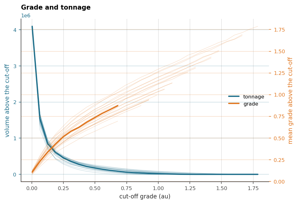
The spread between the thin curves is what the model does not know about the answer, which is the number a competent person actually needs beside the estimate. Chapter 12 takes the same blocks to surfaces and exports, and chapter 14 to the reporting figures.

In the code. data.BlockSet3D and RotatedBlockSet3D, with the criteria needs_splitting, unbalanced and crossed_by, and models.refine as the driver. Design and measurements: docs/variable-block-models.md.

Further reading

Journel & Huijbregts (1978) and Chilès & Delfiner (2012) for the change of support classically; David (1977) for its mining consequences; docs/variable-block-models.md for this implementation’s design record and the measured accuracy of the refinement criteria.

References

Chilès, J.-P., & Delfiner, P. (2012). Geostatistics: Modeling Spatial Uncertainty (2nd ed.). Wiley.

David, M. (1977). Geostatistical Ore Reserve Estimation. Elsevier.

Journel, A. G., & Huijbregts, C. J. (1978). Mining Geostatistics. Academic Press.