3. Inducing points and the ELBO

Chapter 2 ended at the wall. The exact model costs \(\mathcal{O}(N^3)\), and kriging’s classical way around it, the search neighbourhood, buys speed with artefacts, because every target location gets a different model and none of them sees the whole campaign. The variational answer keeps one global model and makes it sparse instead. This chapter is the package’s engine room, and every model in the rest of the manual is built from the pieces introduced here.

3.1 Pseudo-data: the inducing points

Pick \(U \ll N\) locations \(\mathbf{T}\), the inducing points, and let the model carry a distribution over the field’s values \(\mathbf{u}\) at those locations only:

\[ q(\mathbf{u}) = \mathcal{N}(\mathbf{u};\, \mathbf{m}, \mathbf{S}). \]

Everything else is read through them. The prediction at any location is the prior conditioned on \(\mathbf{u}\), averaged over \(q\). The intuition is entirely geostatistical: the inducing values are a composite of the information, a small, well-placed campaign standing in for the full database, with \(\mathbf{m}\) its estimates and \(\mathbf{S}\) how sure it is. The heavy algebra now runs on \(U \times U\) matrices, the cost falls to \(\mathcal{O}(NU^2)\), and \(N\) only enters linearly.

The parameters of \(q\) are not solved for in closed form. They are fitted, by maximizing the evidence lower bound (ELBO):

\[ \log p(\mathbf{z}) \;\ge\; \sum_{n=1}^{N} \mathbb{E}_{q(f_n)}\left[\log p(z_n \mid f_n)\right] \;-\; \mathrm{KL}\left[q(\mathbf{u}) \,\|\, p(\mathbf{u})\right]. \]

That expression is worth walking through slowly, because every training run in this manual is a climb up it.

Two different quantities live at each sample location. \(f_n\) is the value of the latent field at \(\mathbf{x}_n\), the ground itself, which nobody ever observes. \(z_n\) is the measurement, the number in the assay file. They are related by the likelihood \(p(z_n \mid f_n)\), which in the simplest case says \(z_n = f_n + \epsilon_n\) with \(\epsilon_n\) the nugget of chapter 2. Keeping the two apart is not pedantry, and chapter 4 turns it into a working doctrine, but it already earns its keep here: the model is asked to explain the measurements, while what it carries a distribution over is the ground.

The first term is a weighted average, not an evaluation. The model does not know \(f_n\). What it knows is \(q(f_n)\), a Gaussian marginal got by conditioning the prior on \(\mathbf{u}\) and averaging over \(q(\mathbf{u})\). So the fit term cannot be “the likelihood at the estimate”. It is the likelihood averaged over every value the field might plausibly take there, each weighted by how plausible the model currently finds it:

\[ \mathbb{E}_{q(f_n)}\left[\log p(z_n \mid f_n)\right] = \int \log p(z_n \mid f)\; q(f_n = f)\; \mathrm{d}f . \]

This is why the model is honest about its own uncertainty rather than merely reporting it. A location where \(q(f_n)\) is wide contributes a smeared likelihood, and smearing costs. Being uncertain is penalised exactly where the data could have pinned the field down, so widening the posterior to dodge a residual is not free. It also means the term is not generally available in closed form. For a Gaussian likelihood with a linear warping it is, and otherwise geoML computes it by quadrature or by sampling, which is where n_sim and the quadrature node counts of chapter 4 come from.

The second term is the restraint. \(\mathrm{KL}[q(\mathbf{u}) \| p(\mathbf{u})]\) measures how far the fitted \(q\) has moved from the prior, which is the covariance model of chapter 2. It pulls the other way from the fit term, a built-in penalty against fitting noise, playing the role the nugget and the modeller’s restraint play in classical practice. The difference is that here it is part of one objective rather than a convention.

Everything trainable climbs this single number by gradient ascent (Adam): variational parameters, ranges, sill, noise, and the warping.

Two technical choices are worth knowing by name because they appear in every saved model. The variational mean is whitened (\(\boldsymbol{\alpha} = \mathbf{L}^{-1}\mathbf{m}\), with \(\mathbf{K}_{uu} = \mathbf{L}\mathbf{L}^T\)), which decouples it from the kernel parameters during optimization. The covariance uses the Opper–Archambeau form, which adds only \(2U\) parameters and guarantees the posterior variance never exceeds the prior’s. Titsias (2009) and Hensman et al. (2013, 2015) are the source papers.

In the code. The pair geoml.latent.BasicInput (the inducing points and the spatial transform at the door) and geoml.latent.BasicGP (the kernel and the variational state) is the minimal network. geoml.models.VGPNetwork owns the ELBO, train_full and train_svi. The whitened mean and the variance parameters are alpha_white_* and delta_* on each node, which chapter 13 re-initializes to make a fold model forget.

3.2 Feeding it: full batch or stochastic

The ELBO is a sum over samples, so a minibatch of size \(B\) estimates it after rescaling by \(N/B\). That is stochastic variational inference. train_full uses everything at each step and is the right call up to a few thousand samples. train_svi cycles reproducible random batches and is how 18 000 assays train comfortably.

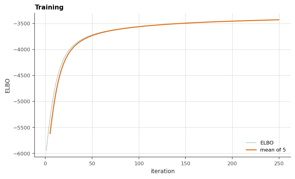
The curve to watch is the same for both. The ELBO trace is noisy by construction, since the expectation above is estimated, so read its running mean: flat means settled, still climbing means keep going. Stopping early is a quiet source of bad maps, and it is cheap to avoid.

3.3 Placing them, and how many

Where the inducing points go is a modelling decision the package makes easy and deliberate:

inducing.from_kmeans(data, n) puts them where the data is, which suits drillhole geometry: dense where the holes are dense.
inducing.from_grid(data, step) covers a region evenly, for when the prediction area matters more than the sampling.

Their positions are then fixed. That is a design decision rather than a limitation. Trainable positions were tested and rejected, because points wander away from the region of interest and get stuck, and coverage is worth more than the marginal likelihood gain. What is trainable is everything the points carry.

How many is the model’s main capacity knob, and the reading is the variogram’s. A smooth field is summarized by few, one or two hundred, while a short-range, high-nugget field needs many to have anything local to say. Too few shows up as an over-smoothed map that misses the highs.

Too many mostly costs time, and it is worth being exact about what it does not cost. Here is the plainest version of this dataset — 259 Jura samples, a stationary model with a Gaussian likelihood, everything held but the inducing count, scored on the 100 sites nobody trained on:

inducing points	rmse / sd	90% coverage	predicted sd / data sd
81	0.935	0.936	0.917
169	0.930	0.926	0.873
324	0.927	0.911	0.839
625	0.932	0.894	0.804

The accuracy does not move across nearly eight times the capacity. What moves is the width of the model’s own uncertainty: the intervals narrow, carrying a nominal 90% band from mildly conservative to mildly optimistic. That drift is the thing to watch, and at this size it is not a reason to hold back — a model covering 0.89 where it promised 0.90 is a calibrated model.

How that table is read matters more than the table, because reading it wrong manufactures an alarming version of the same numbers. predict reports the ground, with the likelihood’s noise averaged out, so the simulations it stores describe a quantity no sample observes. Score those directly against assays — which is what compute_metrics() on the predicted container does — and the noise is missing from every interval: the 90% band above then reads 0.59 falling to 0.49 rather than 0.94 falling to 0.89, and the error grows with capacity, because a model with more capacity explains more of the variation as field and less as noise, so the omitted piece gets bigger. Chapter 13 develops this properly; the short version is that intervals of a measurement come from predict_measurements, which is what the accuracy figure and cross_validate both use.

There is a tidy story about the kernel range here that does not survive being checked, and it is worth knowing that it does not. The range is a plain point estimate the objective never charges for, so one expects that as capacity grows the field is free to roughen — and the fitted range does fall, 3.9 km to 2.7 km, straight down that table. But freezing it at the value the smallest model chose makes the calibration worse at every count. The shrinking range is the model compensating, not the model failing.

So the count is a knob with no safe default, and there is only one way to set it: measure on data the model has not seen, for the configuration you actually intend to use, with intervals of the right quantity. Both case studies do exactly that, and show their tables.

3.4 Experts: many small models, one answer

Past a few hundred inducing points the \(U^3\) work inside the model starts to bite, and the answer is the geostatistical instinct again: local models. The inducing set is split into overlapping experts, each a small set responsible for its region, combined by precision weighting so that no seam shows where one hands over to the next.

inducing.grid_experts(data, step, block=4) lays the experts out as overlapping blocks of a lattice. Every expert holds the same number of points, which keeps the model’s internal state rectangular.
inducing.experts(from_kmeans(data, 1500), 12) is the unordered version: clustered experts that follow the data, each borrowing a share of its neighbours’ points.

With many experts, one option matters. GPOptions(expert_propagation="independent") lets each expert speak for its own inducing set alone, instead of all experts cross-predicting each other ("consensus", the default). Measured on this package, training runs 1.6× faster at 5 experts and 6.3× at 40, prediction up to 8×, with quality within a few percent either way. Past roughly ten experts the consensus is paying a quadratic bill for a cosmetic agreement.

3.5 Walker Lake, sparse

Now chapter 2’s model rebuilt the modern way. The inducing points are laid on a 10-unit lattice covering the prediction grid rather than the samples, because the model has to say something everywhere the grid asks, including the gaps between the sampled lines. grid_experts cuts that lattice into blocks and returns one set per expert.

import os

import geoml

os.makedirs("figures", exist_ok=True)
geoml.set_seed(1234)

walker, walker_grid = geoml.datasets.walker()

# one node every 10 units over the grid's extent, cut into blocks of
# 8 x 8 nodes; each expert also takes one node of margin all around, so
# neighbouring experts overlap and their answers blend without a seam
experts = geoml.data.inducing.grid_experts(walker_grid, 10.0, block=8)
print(len(experts), "experts of", experts[0].n_data, "inducing points")

root = geoml.latent.BasicInput(
    experts,
    transform=geoml.transform.Isotropic(50))

gp = geoml.latent.BasicGP(
    root,
    size=1,
    kernel=geoml.kernels.Spherical())

model = geoml.models.VGPNetwork(
    walker, "V",
    geoml.likelihood.Gaussian(geoml.warping.ZScore(1)),
    gp,
    options=geoml.models.GPOptions(verbose=False))

model.train_full(max_iter=250)

figure = geoml.plots.Explorer(walker, continuous="V",
                              model=model).training_curve()
figure.savefig("figures/03-training-curve.png", dpi=150,
               bbox_inches="tight")

The ELBO trace and its running mean

import matplotlib.pyplot as plt

model.predict(walker_grid, n_sim=20)
walker_grid.get("V").reset_quantiles([0.5])

figure, axes = plt.subplots(figsize=(5, 4.5))

drawn = axes.imshow(walker_grid.get("V/quantiles/0.5").as_image(),
                    origin="lower", cmap="cividis")
figure.colorbar(drawn, ax=axes, shrink=0.85)
axes.set_title("median, %d experts" % len(experts))

figure.savefig("figures/03-walker-sparse.png", dpi=150,
               bbox_inches="tight")

The sparse model's median map

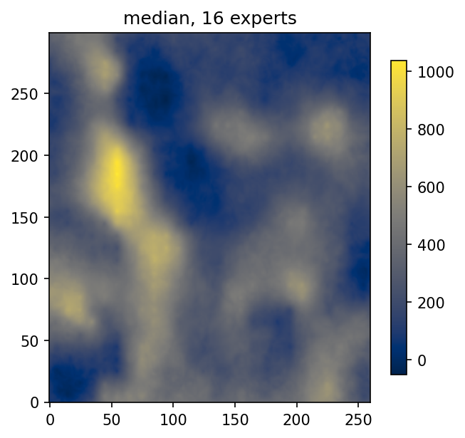
This is chapter 2’s map. The same highs in the same places, the same lows between them, and the same defect: nothing prevents a negative grade, because the model is still a Gaussian field behind a linear warping. The peaks are a little flatter, since the inducing points do not sit on the samples and a lattice at 10 units cannot resolve a spike narrower than that. Beyond it, the sparse construction did not change the answer, which is the point being made here. It changed what the model is able to become.

Nothing was gained in speed on 470 samples, and nothing should have been. What the inducing points buy is room. Everything the following chapters add (a trainable warping that keeps grades positive, a categorical variable sharing the same network, a second layer that bends space, a block model refined where the cut-off is undecided) rides on a model whose cost no longer grows with the cube of the sample count. On this dataset that is a promise. On a real campaign it is the difference between a model and no model.

References

Gonçalves, Í. G. et al. (2022). Learning spatial patterns with variational Gaussian processes: regression. Computers & Geosciences. https://doi.org/10.1016/j.cageo.2022.105056

Gonçalves, Í. G. et al. (2026). Scalable variational Gaussian process framework for implicit geological modelling and compositional grade interpolation. Artificial Intelligence in Geosciences. https://doi.org/10.1016/j.aiig.2026.100218

Hensman, J., Fusi, N., & Lawrence, N. D. (2013). Gaussian processes for big data. Proceedings of the 29th Conference on Uncertainty in Artificial Intelligence (UAI), 282–290.

Hensman, J., Matthews, A. G. de G., & Ghahramani, Z. (2015). Scalable variational Gaussian process classification. Proceedings of the 18th International Conference on Artificial Intelligence and Statistics (AISTATS), 351–360.

Opper, M., & Archambeau, C. (2009). The variational Gaussian approximation revisited. Neural Computation, 21(3), 786–792.

Titsias, M. K. (2009). Variational learning of inducing variables in sparse Gaussian processes. Proceedings of the 12th International Conference on Artificial Intelligence and Statistics (AISTATS), 567–574.