9. From database to data

Models see points, and a mine keeps collars, surveys and interval tables. DrillholeData is the bridge, and it is deliberately a one-way one. It desurveys, validates, composites and converts, but it is never fed to a model. Only what it produces is. That separation keeps the database manipulations, which must be auditable, apart from the modelling, which must be fast, and it is why the class leans on pandas while everything downstream leans on arrays.

9.1 Ingesting: rename at the door

The constructor takes the collar table, optionally a survey, plus the names your database uses, and renames everything to canonical columns on the way in. Whatever the file called them, holes become HOLEID and intervals become FROM/TO. Reaching for the original names afterwards is a deliberate KeyError: one spelling inside the package, however many outside. Interval tables join by name, each with per-column roles declared once: grade (composited by length × density when a density column is declared), categorical, density, recovery (composites by length, never weights a grade, converts to metadata), flag and ignore.

A column may also declare what it is measured in — units={"Pb": "%", "Ag": "ppm"} at construction, or afterwards on a database somebody else built:

holes.set_unit("assay", {"Pb": "%", "Ag": "g/t"})

That declaration travels with the column through renaming and compositing and lands on the variable the conversion builds. On an ordinary grade it is a label, naming an axis and riding an export; on a part of a composition it is the number the part is divided by, which is the subject of §9.4. Validation reports a value above the whole its unit measures — 120 in a column called a percentage — because that is the shape a mislabelled unit takes.

Declare the units before compositing. set_unit changes the table the database holds, in place, and a composite is a new object: it carries the units it was given but no longer shares them.

Desurveying is minimum curvature, with a straight-line fallback along the collar attitude and a warning when a hole has neither. Interval coordinates are never stored. They are computed on demand, which is what keeps compositing exact instead of accumulating rounding.

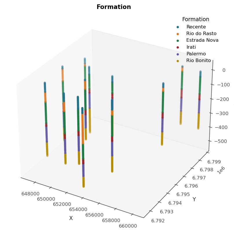
The bundled Araranguá set shows the shape of it: 13 vertical holes and one lithology table.

import os

import geoml

os.makedirs("figures", exist_ok=True)

holes = geoml.datasets.ararangua()
print(holes)

9.2 Compositing: one support before anything else

Assays come at the lengths the geologist cut, and mixed supports are a quiet bias, because a long rich interval and a short poor one are not two equal votes. Compositing regularizes the support, and the class offers three deliberate flavours:

composite(length, domain="litho") is the default, honouring domain boundaries so that no composite straddles a contact;
composite_fixed(length) uses a fixed length regardless;
composite_to("assay") puts every table onto one table’s support, which is what makes the point conversion a one-to-one merge.

Each returns a new DrillholeData with every table on the shared support. On a real assay database the round trip reproduces the assays to about 1e-13, and a hand-computed mass-weighted composite matches exactly. The tests pin both.

9.3 Converting: what the models actually receive

as_point_data() produces the PointData the models take, and every conversion carries three columns as metadata, which are per-location facts the models never see: the hole id (HOLEID), the depth down the hole (DEPTH) and the sample length (LENGTH). The identifier is what leave-one-hole-out validation splits on (chapter 13), the length is what a weighting scheme reads, and the depth is what a contact profile measures from: Explorer.contact puts a grade against its distance down the hole to the nearest contact between two domains, which is the figure the hard-or-soft boundary decision is read from before anything is modelled. This database logs no assays, so the chapter cannot draw one. All three travel with the data through subsetting, prediction and Zarr, and none is modelled.

For categories, the conversion of chapter 6 gives interior points plus the contacts between domains, the latter carrying both neighbouring classes at zero support:

point = holes.as_classification_input(("lito", "Formation"), length=5.0)
print(point.tree())

print(point.n_data, "points from",
      len(set(point.get_metadata("HOLEID"))), "holes")

The table carries three categorical columns (Lito, Formation, Layer), so the conversion asks for the one it should model rather than guessing, as the error message tells you if you let it.

figure = geoml.plots.Explorer(point, categorical="Formation").scene()
figure.savefig("figures/09-ararangua-classification.png", dpi=150,
               bbox_inches="tight")

The classification input: interior points and contacts

9.4 Compositions: several metals, one whole

A composition is a set of parts that share a whole, and the whole is what makes a log-ratio transform meaningful. Assays do not arrive that way: lead is reported in percent, silver in grams per tonne, and the two cannot be added up until both are fractions of the same rock. That is why a compositional group is declared with its units.

metals = holes.as_point_data(
    compositional={"metals": {"columns": ["Pb", "Ag"], "rest": True}})

With the units on the table, the group names its columns and nothing else. Where the table declares none, name them in the group itself — {"columns": {"Pb_pct": "%", "Ag_ppm": "ppm"}, "rest": True} — and a part left undeclared is read as a fraction, with a warning saying so. This database logs no assays, so the code above is written out rather than run; the bundled Arctic lake set is a composition and shows what comes of it.

Three things happen on the way in. A row missing any one part is marked missing entirely, since the parts only carry information relative to each other. Non-positive values are replaced by half the smallest positive value of their own column, the usual substitution below detection, because a log-ratio cannot take a zero. And the row is closed: with rest=True a further part is added holding whatever is left of the whole, which is the one to reach for when the parts are a few assayed metals, because their own numbers then survive untouched. Closing without a rest turns them into shares of what was measured instead.

The parts keep their units. Lead stays in percent everywhere you look at it — its prediction, its realizations, its quantiles, its dispersion inside a block, the scatter a fresh sample would show. Only at the two doors where the model reads and writes does it become a fraction of the whole, which is where it has to be one. A cut-off is declared in the part’s own unit for the same reason. The container will tell you what it is holding, and the variable will show you both sides:

lake = geoml.datasets.arctic_lake()
print(lake.units())

sediment = lake.get("comp")
print("stored, as logged:", sediment.values("Sand/measurements")[:3])
print("as the model reads it:", sediment.get_measurements()[0][:3])

The first row is percentages, the second the same three numbers as fractions of one whole. Nothing but the doors ever sees the second.

In the code. geoml.data.DrillholeData and IntervalTable in data/drillhole.py: add_intervals, set_role, set_unit (on the table for one column, on the database for a whole table), rename, rename_table, drop_table, the three composites, as_point_data(position=, drop_missing=), get_contacts and as_classification_input. One sign-convention gotcha the constructor exposes as dip_positive_down: geoML reads a positive dip as downward, and many databases record downward holes as negative. Getting it wrong mirrors every hole through its collar, which is obvious in a 3D view and invisible in a summary, so look at the traces before modelling anything.

References

Abzalov, M. (2016). Applied Mining Geology. Springer.

Gonçalves, Í. G. et al. (2023). Variational Gaussian processes for implicit geological modeling. Computers & Geosciences. https://linkinghub.elsevier.com/retrieve/pii/S0098300423000274