16. Case study: Jura

Seven correlated heavy metals and a rock type, 259 training sites and 100 held out. This is the classic multivariate testbed, and the case study for one model carrying two variables of different kinds at once, where one of them is allowed to inform the other. The payoff of sharing a model is not elegance. The rock type and the metals share spatial structure, and a network that lets them say so predicts both better than two models that cannot.

16.1 Look, jointly

import os

import geoml
import matplotlib.pyplot as plt

os.makedirs("figures", exist_ok=True)
geoml.set_seed(1234)

jura_train, jura_validation = geoml.datasets.jura()
print(jura_train.tree())

elements = list(jura_train.get("Elements").labels)
rocks = list(jura_train.get("Rock").labels)
print(elements)
print(rocks)

explore = geoml.plots.Explorer(jura_train, continuous="Elements",
                               categorical="Rock")

explore.histogram().savefig("figures/16-histograms.png", dpi=150,
                            bbox_inches="tight")
explore.pairs(kind="scatter").savefig("figures/16-pairs.png", dpi=150,
                                      bbox_inches="tight")

Seven metals, grouped by rock

The metals against each other

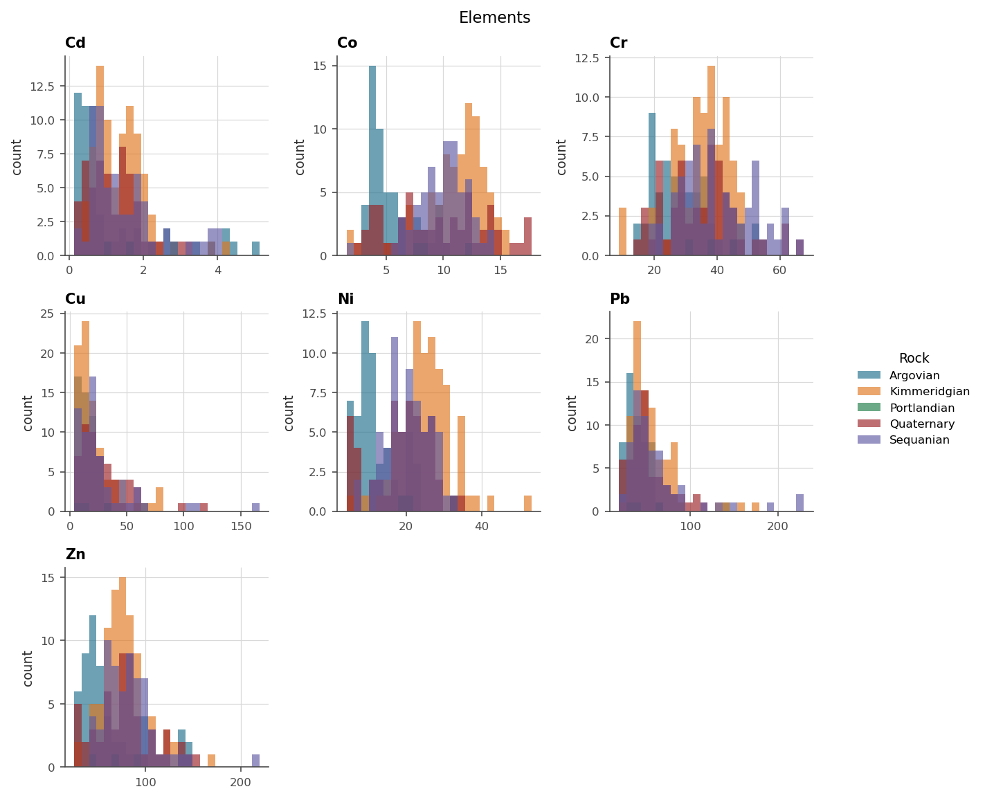
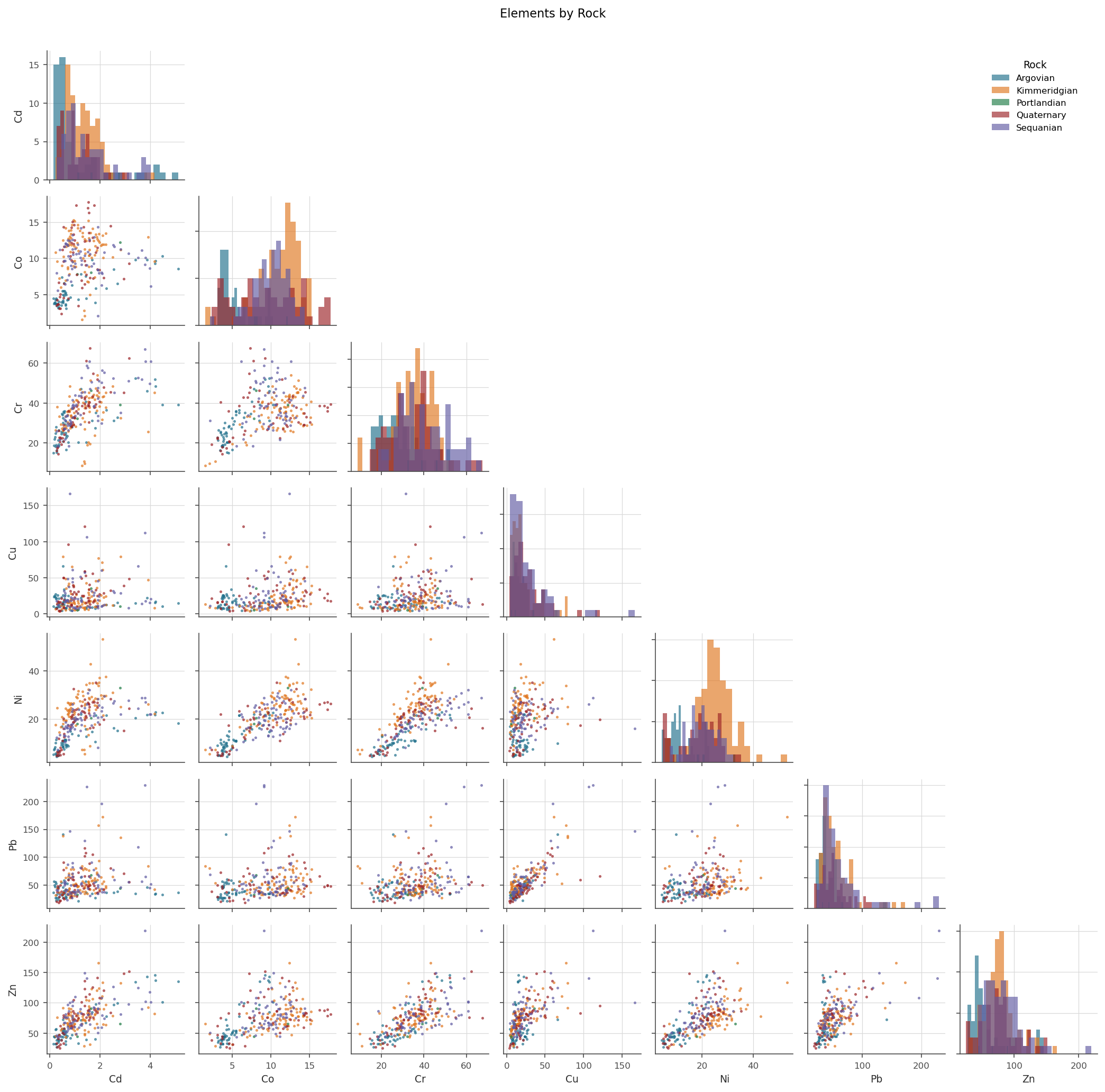
Two arguments for the joint model, both visible before any modelling. The histograms grouped by rock type show several metals shifting distribution with the geology, so the rock type is informative about the grades. The pair plot shows the metals are strongly correlated with each other and skewed, which is what the warping chain below has to deal with.

16.2 A non-stationary network, and how one variable reaches another

The network is the whole point of this chapter, so it is built in three pieces with the reason for each said out loud.

The inducing points are the data’s own locations plus a regular backbone, so that the model is anchored where the samples are and still has something to say over the empty parts of the map. They are then divided into experts (chapter 3).

grid = geoml.data.Grid2D(start=[0, 0], end=[6, 6], n=[201, 201])

backbone = geoml.data.inducing.combine(
    jura_train,
    geoml.data.Grid2D(start=[0, 0], end=[6, 6], n=[21, 21]))

inducing = geoml.data.inducing.experts(backbone, 4)

print(backbone.n_data, "inducing points, split into", len(inducing),
      "experts holding", sum(part.n_data for part in inducing),
      "between them")

root = geoml.latent.BasicInput(
    inducing_points=inducing,
    transform=geoml.transform.Isotropic(0.05))

The two counts differ because the experts overlap: each borrows a share of its neighbours’ points so that they blend rather than butt up against each other (chapter 3). The 700 is the number of distinct locations; the larger number is what the four sets hold between them. The blending is good but not perfect. A faint trace of the expert boundaries is visible in the uncertainty map at the end of this chapter, which is the most sensitive column to look for it in.

The geology is modelled in a space the model is allowed to bend. An inner GP of two columns moves the coordinates, GPWalk integrates that movement over a few steps, and the rock-type fields are modelled on the result. A stationary kernel in the moved space is a non-stationary one in the real space, which is chapter 5’s argument applied to a contact rather than to a grade.

displacement = geoml.latent.BasicGP(
    root, size=2, kernel=geoml.kernels.Gaussian())

walked = geoml.latent.GPWalk(displacement, n_steps=5)

rock_gp = geoml.latent.BasicGP(
    walked, size=len(rocks), kernel=geoml.kernels.Matern32())

The geology reaches the grades as a trend that is added to them. A Linear node takes the five rock fields to seven columns, one per element, and LinearCombination adds that to a GP of the metals’ own. The unit_norm=False is the important argument: it lets the mixing weights shrink towards zero, so the model can decide that the geology says nothing about a particular element rather than being forced to use it.

trend = geoml.latent.Linear(
    rock_gp, size=len(elements), unit_norm=False)

metal_gp = geoml.latent.BasicGP(
    root, size=len(elements), kernel=geoml.kernels.Spherical())

# the model's output: rock indicators first, then the metals, matching the
# order of the variables and likelihoods below
network = geoml.latent.Concatenate(
    rock_gp,
    geoml.latent.LinearCombination(trend, metal_gp))

That is a different move from making the rock fields a parent of the metal GP. Both are available, and the difference is how strong a claim they make. A parent would have the metals read the geology through the uncertainty propagation of a deep GP, committing to the grades living in the geology’s warped space. The additive trend says something weaker and more defensible: whatever the rock type contributes, add it, and let the weights decide how much.

The likelihood is where the metals’ awkwardness is handled. Laplace has heavier tails than a Gaussian, which is what the extreme values in this dataset want, and the chain does the rest: Log for non-negativity, RobustPCA to decorrelate the seven columns, Spline for what asymmetry is left, and ZScore to hand the field something standardized.

warping = geoml.warping.ChainedWarping(
    geoml.warping.Log(len(elements)),
    geoml.warping.RobustPCA(len(elements), len(elements)),
    geoml.warping.Spline(len(elements), knots_per_arm=5),
    geoml.warping.ZScore(len(elements)))

model = geoml.models.VGPNetwork(
    data=jura_train,
    variables=["Rock", "Elements"],
    likelihoods=[
        geoml.likelihood.CategoricalGaussianIndicator(len(rocks)),
        geoml.likelihood.Laplace(warping=warping)],
    latent_network=network,
    options=geoml.models.GPOptions(prediction_batch_size=1000,
                                   jitter=1e-6, verbose=False))

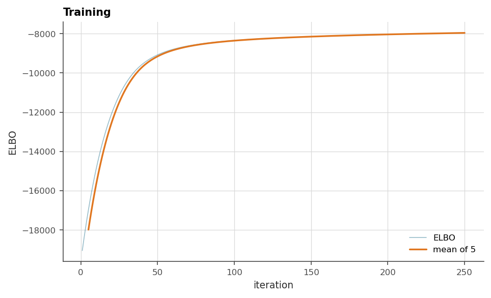
model.train_full(250)

figure = geoml.plots.Explorer(jura_train, continuous="Elements",
                              model=model).training_curve()
figure.savefig("figures/16-training.png", dpi=150, bbox_inches="tight")

The ELBO, with two variables pulling on it

16.3 How many inducing points, and how we know

The inducing set above is larger than the score needs, and rather than assert that, here it is measured. Everything below is the same network, the same warping and the same 250 iterations, with only the inducing points changing, scored on the 100 sites nobody trained on. The metals’ error is divided by each element’s own standard deviation and averaged, so 1.0 would mean “no better than quoting the average grade”.

inducing points	training	metals, rmse / sd	goodness	rock accuracy
259, the data alone	54 s	0.90	0.47	0.73
380, data + an 11 × 11 backbone	66 s	0.90	0.50	0.73
700, data + 21 × 21, four experts	198 s	0.90	0.51	0.72
1220, data + 31 × 31, four experts	300 s	0.91	0.48	0.71

The score does not move. Nearly five times the inducing points, five and a half times the training, and the held-out error is flat to the second decimal.

Chapter 3 ran the same sweep on the plainest possible version of this dataset — a stationary model, a Gaussian likelihood, no walked input — and found the same flatness, from 81 inducing points to 625. Two configurations this far apart agreeing is worth more than either alone: what capacity buys is resolution rather than accuracy at the sampled sites, and what it costs is a slow narrowing of the model’s own intervals, which a validation table shows long before it becomes a problem. The goodness column above is computed from the container’s stored simulations, so like every such number it describes the ground rather than an assay and reads low; chapter 13 does it the honest way, and cross_validate does it that way for you.

So why keep the larger set? Because the table is measured at sampled locations, and it cannot speak for the ground between them. A regular backbone of inducing points exists for the map, and a validation set drawn from the same campaign is structurally unable to notice it. That is a limit of the metric rather than a verdict on the backbone, and it is the kind of blind spot worth naming: a number that does not move is not always a number that has looked.

Where the table is decisive is cost. If you want this model and not its map, the data’s own locations give the same score in a quarter of the time.

16.4 Did the warping do its job?

The model assumes its latent columns are independent standard normals. The warping is what has to deliver that, and it is easier to look at than to test.

figure = geoml.plots.Explorer(jura_train, continuous="Elements",
                              model=model).transformed_pairs(upper="density")
figure.savefig("figures/16-transformed.png", dpi=150, bbox_inches="tight")

The metals as the model sees them

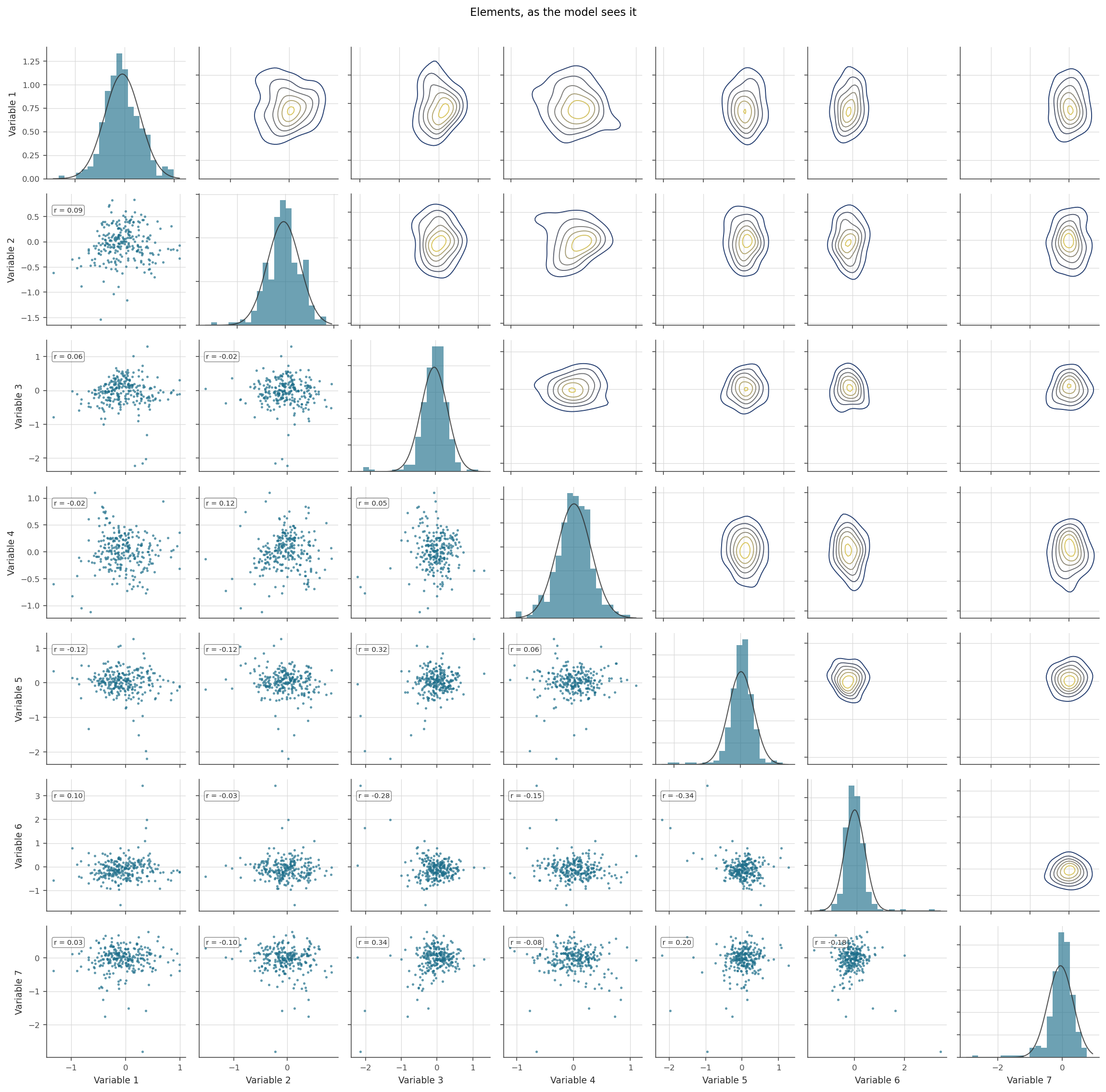
Down the diagonal, each column should sit under the standard normal drawn over it. Off the diagonal, the clouds should be round and the correlations near zero. The columns are numbered rather than named, because after a rotation a column is a mixture of the measured elements rather than any one of them. Leaning clouds here are dependence the model is about to assume away, which is the argument for keeping RobustPCA in the chain.

16.5 Score on the samples nobody trained on

Jura ships with a genuine held-out set, so scoring is one prediction away, and the accuracy figure is honest here without any cross-validation (chapter 13’s caveat does not bite on a true validation set).

model.predict(jura_validation, n_sim=30, include_noise=True)

metal_scores = jura_validation.get("Elements").compute_metrics()
print(metal_scores.loc[["Root Mean Square Error (prediction)",
                        "CRPS (simulations)",
                        "Goodness (simulations)"]].round(3))

rock_scores = jura_validation.get("Rock").compute_metrics()
print(rock_scores.round(3))

explore = geoml.plots.Explorer(jura_validation, continuous="Elements",
                               model=model)

explore.accuracy().savefig("figures/16-accuracy.png", dpi=150,
                           bbox_inches="tight")
explore.simulation_pairs().savefig("figures/16-simulation-pairs.png",
                                   dpi=150, bbox_inches="tight")

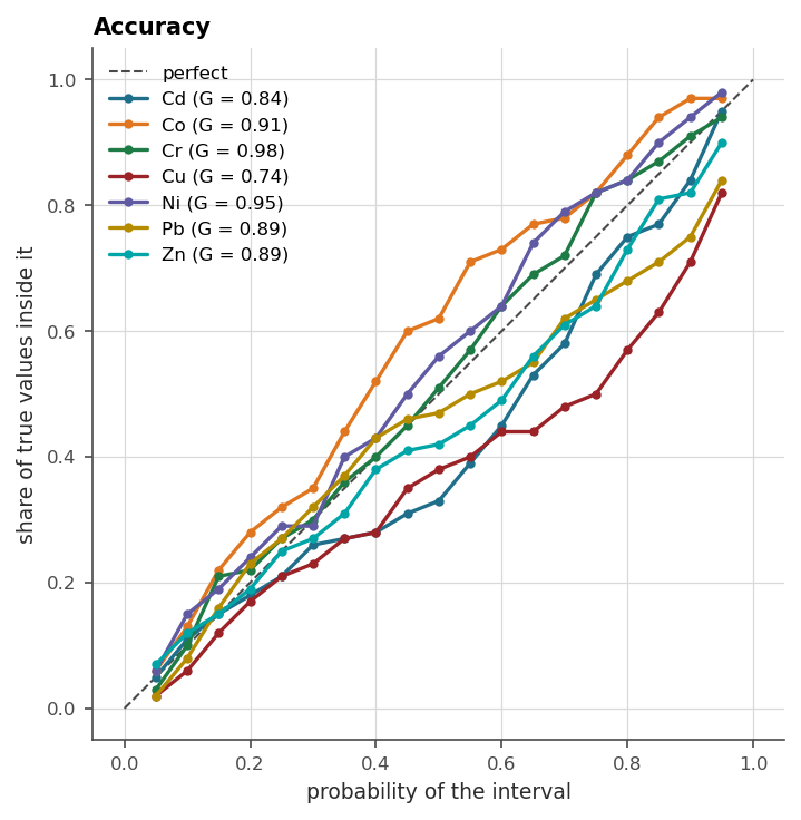
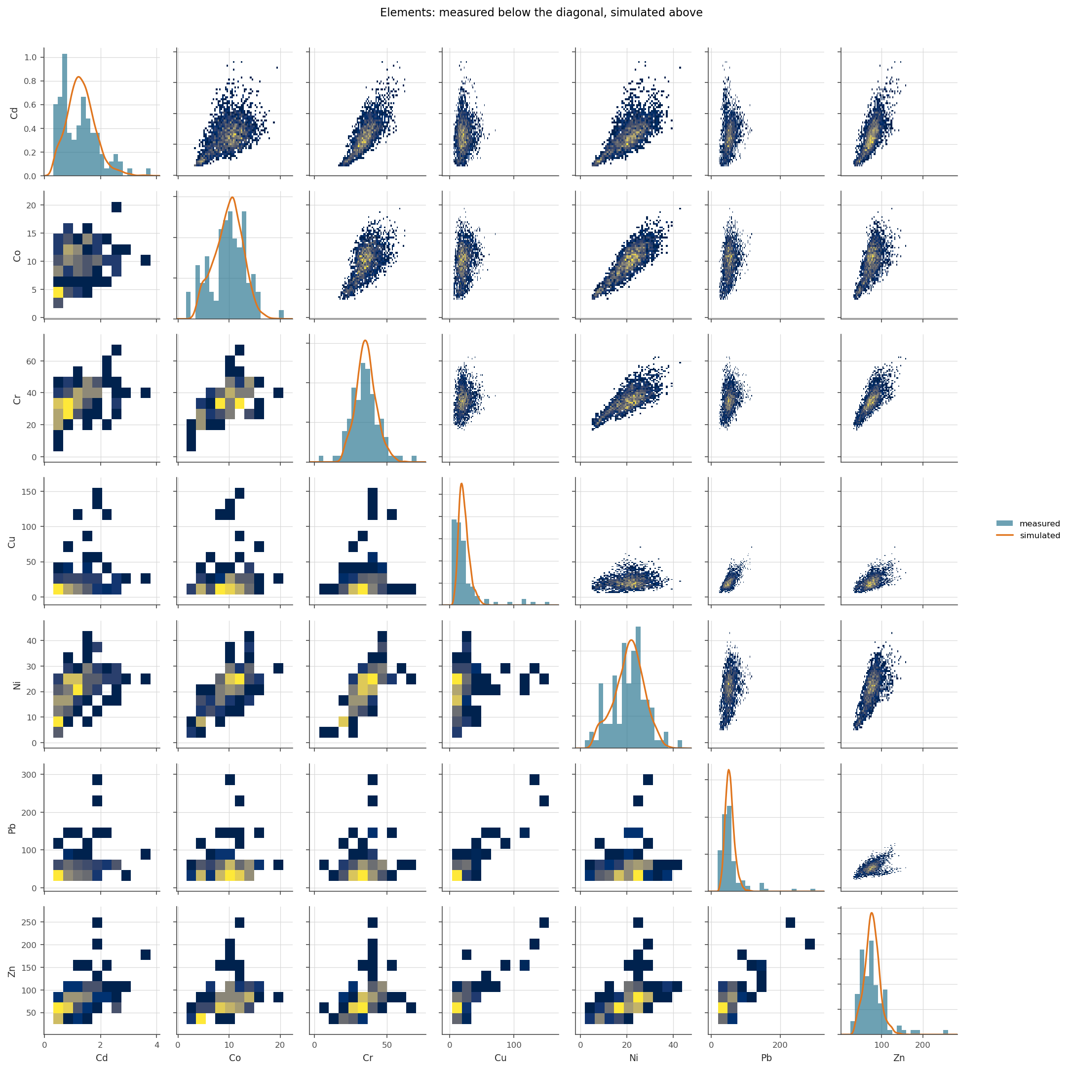
Every element's interval claim, checked

The simulated joint distribution against the measured one

compute_metrics reports per component: seven columns for the metals, and balanced accuracy and friends per rock class. That is the table a report wants, and the accuracy figure is its calibration column drawn.

One column in the rock table is worth reading before it is mistaken for a bug. Portlandian comes back with a balanced accuracy of 0.5 and a Jaccard of zero, which is what those statistics say about a class the model never predicts anywhere. It is the rarest formation in the training set, the other four outvote it at every location, and no amount of fitting will change that without telling the model the class matters more than its frequency suggests. A rare domain that matters is a modelling decision, not a scoring accident.

simulation_pairs asks the question a per-variable score cannot. The realizations should reproduce not only each metal’s own histogram but the shape of the cloud every pair of them makes. A model that gets the margins right and the joint wrong will estimate any function of two metals badly, and a smelter payment schedule is exactly such a function.

16.6 Map everything

One prediction over the grid fills both variables at once.

model.predict(grid, n_sim=30, include_noise=True)
grid.get("Elements").reset_quantiles([0.5])

figure, axes = plt.subplots(2, 4, figsize=(14, 7.4))

for ax, element in zip(axes.ravel(), elements):
    # a quantile of thirty realizations is grainy; `sigma` smooths what the
    # figure shows without touching anything stored
    image = grid.get("Elements/%s/quantiles/0.5" % element).as_image(sigma=1)
    drawn = ax.imshow(image, origin="lower", cmap="cividis",
                      extent=(0, 6, 0, 6))
    figure.colorbar(drawn, ax=ax, shrink=0.8)
    ax.set_title(element)

axes.ravel()[-1].set_visible(False)
figure.suptitle("median grade, one model")
figure.tight_layout(rect=(0, 0, 1, 0.94), h_pad=2.5)
figure.savefig("figures/16-element-maps.png", dpi=150,
               bbox_inches="tight")

All seven metals

figure, axes = plt.subplots(2, 3, figsize=(11, 7.4))

for ax, rock in zip(axes.ravel(), rocks):
    image = grid.get("Rock/%s/probability" % rock).as_image()
    drawn = ax.imshow(image, origin="lower", cmap="cividis",
                      extent=(0, 6, 0, 6), vmin=0, vmax=1)
    figure.colorbar(drawn, ax=ax, shrink=0.8)
    ax.set_title("P(%s)" % rock)

last = axes.ravel()[-1]
drawn = last.imshow(grid.get("Rock/uncertainty").as_image(),
                    origin="lower", cmap="magma",
                    extent=(0, 6, 0, 6), vmin=0, vmax=1)
figure.colorbar(drawn, ax=last, shrink=0.8)
last.set_title("uncertainty (entropy)")

figure.suptitle("the geology, and how sure it is")
figure.tight_layout(rect=(0, 0, 1, 0.94), h_pad=2.5)
figure.savefig("figures/16-rock-maps.png", dpi=150, bbox_inches="tight")

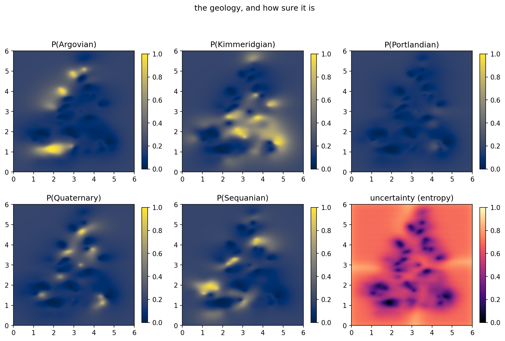
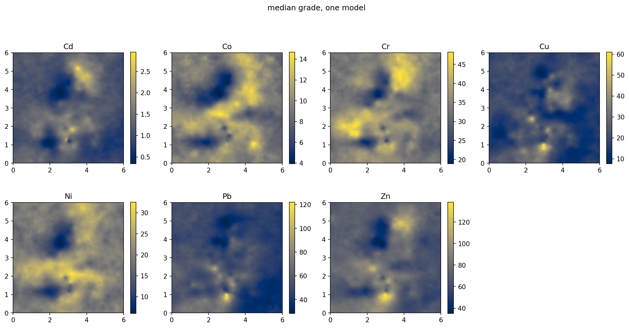
The five formations and the doubt between them

The grade maps and the geology maps came out of one model, and their agreement is not a coincidence to check but a property of the construction. The metal fields carry a trend read off the rock fields, so a formation boundary is visible in the grades because the model was told it might be, and the entropy map marks exactly the places where that reading is least certain.

The sigma=1 in the grade maps deserves a word, since it is the one place this chapter touches a picture rather than a number. A quantile of thirty realizations is a noisy estimate, and as_image(sigma=...) blurs what the figure shows without altering anything the container holds. One pixel is a light touch: it takes the harshest speckle off and leaves the grain, which is the right amount, because that grain is not a rendering artefact. It is the Monte Carlo error of thirty realizations, and a larger sigma would make these maps look more certain than the model is.

That is the rule for the argument generally. It is a presentation choice, fine for a map somebody looks at, and never to be applied to numbers being scored. The maps above go through it and every score in §16.5 does not. The uncertainty map is drawn unsmoothed for the same reason, which is also why the faint cross of the expert boundaries is still visible in it.

References

Goovaerts, P. (1997). Geostatistics for Natural Resources Evaluation. Oxford University Press.

Gonçalves, Í. G. et al. (2022). Learning spatial patterns with variational Gaussian processes: regression. Computers & Geosciences. https://doi.org/10.1016/j.cageo.2022.105056

Gonçalves, Í. G. et al. (2025). Uncertainty propagation in deep Gaussian process networks. Mathematical Geosciences. https://doi.org/10.1007/s11004-025-10187-4