13. Validation
A model scored on its own training data flatters itself, and on spatial data the flattery survives the usual defence. A random k-fold split puts most held-out samples next to a training sample, and on a drillhole dataset usually in the same hole, and a spatial model answers those by proximity rather than by understanding. The scores come out excellent, the block model built from the same fit does not, and the difference was never going to show, because the validation asked an easier question than the mine does. The mine asks about ground between and beyond the holes.
This chapter is the package’s answer, in three moves: build folds that ask the mine’s question, score the model only where it never looked, then repair what the scores say is miscalibrated. Everything runs on the same machinery. A metadata column names the folds, one function drives the cross-validation, and the calibration reads what it leaves behind.
The worked example is the Walker Lake model of chapter 11, trained long enough to have settled. Its Box-Cox link is shifted by one before the power, and §13.3 shows the validation that called for it.
import os

import geoml
import numpy as np

os.makedirs("figures", exist_ok=True)
geoml.set_seed(1234)

walker, walker_grid = geoml.datasets.walker()

experts = geoml.data.inducing.grid_experts(walker_grid, 10.0, block=8)

root = geoml.latent.BasicInput(
    experts,
    transform=geoml.transform.Isotropic(50))

gp = geoml.latent.BasicGP(
    root,
    size=1,
    kernel=geoml.kernels.Spherical())

# shifted by one, the order of the smallest grade, so the zeros have a
# logarithm near the rest of the data rather than far below it
warping = geoml.warping.ChainedWarping(
    geoml.warping.BoxCox(1, shift=1.0),
    geoml.warping.ZScore(1))

model = geoml.models.VGPNetwork(
    walker, "V",
    geoml.likelihood.Gaussian(warping),
    gp,
    options=geoml.models.GPOptions(verbose=False))

model.train_full(max_iter=500)
13.1 Folds that mimic the prediction task
What decides how hard a location is to predict is how far its nearest
training sample sits. A useful validation therefore reproduces the
distance geometry of the real task. Held-out samples should be as far
from the training data as the block model’s locations are from the
samples: no nearer, or the scores flatter, and no farther, or the
validation tests an extrapolation nobody asked for. This is the
nearest-neighbour distance matching idea (Linnenbrink et al., 2024), and
geoML holds an advantage the ecology literature it comes from does not.
The prediction target is not a guess. It is the grid or block model in
your hands, and spatial_k_fold takes it as its first argument.
w, target, achieved = walker.spatial_k_fold(walker_grid, k=5, seed=0)
print("W =", round(w, 2))
The method gathers the samples into small groups that are never split
across folds, agglomerates them by cutting a dendrogram of group centroids
at every possible count, and keeps the cut whose held-out-to-training
distance distribution best matches the target’s. That match is the
Wasserstein distance W, in coordinate units, and zero would be perfect.
The folds land in a metadata column named "fold", and the two returned
distance samples let you look at the match instead of trusting it.
Two arguments matter in practice.
groups="HOLEID"names a metadata column whose labels must never be split. On drillhole data this is not optional. Samples from one hole are near-duplicates, and a fold boundary through a hole leaks like a sieve. Every conversion fromDrillholeDatacarries the hole id as metadata for exactly this reason (chapter 9).name=renames the output column, so two labellings can sit side by side and be compared on theirW.
Leave-one-hole-out needs no builder at all. Point the next section’s
folds= argument straight at the hole-id column, and each hole becomes a
fold of its own.
13.2 Scoring where the model never looked
Classical kriging cross-validates cheaply, because the solution is a
closed form and removing one sample and re-solving costs little (Rasmussen
& Williams, 2006, §5.4.2, is the GP spelling of the same trick). The
variational model’s posterior is fitted rather than solved, and
retraining it from scratch once per fold is the cost this package refuses.
cross_validate is the translation of what kriging practice actually
does, which is to cross-validate with the variogram held fixed.
The trained model is saved once, and each fold gets a copy rebuilt around the data with that fold removed.
The copy’s variational state, the part of a trained model that encodes the data, is re-initialized. That makes it structurally ignorant of the held-out samples, and everything else (kernel, warping, noise) is frozen.
A short refit fits the state to the reduced data, and the held-out rows are predicted into one shared container. The folds partition the data, so the loop ends with every sample predicted by the one model that never saw it.
oof, scores = geoml.models.cross_validate(model, iterations=200, n_sim=20)
print(scores[scores["fold"] == "all"])
Why re-initialize rather than warm-start and let the fold “forget” its
held-out samples? Because forgetting was measured and found wanting. On
this very dataset, warm-started fold models score better than an honest
from-scratch retrain, an edge no honest scheme can have, which makes it
the residual memory of the held-out data, still there after hundreds of
iterations. Fresh initialization matches the honest retrain within a few
percent at a fraction of the cost. The concession that remains, that the
hyperparameters and warping were fitted on all the data, is the same one
kriging makes when it keeps the variogram. The measurements are in
docs/cross-validation.md, and refit="all" trades the other way when
you want it.
Freezing parameters does not make an iteration cheaper: a fold refit still
costs the whole reduced data set per step, whatever is on the tape. So a
model too large to train full-batch is too large to cross-validate that
way, and method="svi" refits each fold in minibatches instead, of the
size the model’s own options already carry. The passes are counted by
epochs rather than iterations, because an epoch is one visit to the
data and therefore many gradient steps — the same distinction as
train_full against train_svi in chapter 11.
oof, scores = geoml.models.cross_validate(
    model, method="svi", epochs=30, n_sim=20)
The score table reads like a drill campaign report, with one row per
variable component and fold, plus a pooled "all" row.
rmse,maeandbiasare point errors of the predictive mean. Bias is prediction minus truth, so positive means overestimation.crpsis the proper score for a distribution against a measured value. It rewards putting probability near the truth and punishes both hedging and false precision, on the scale of the variable, and it reduces to the absolute error for a point prediction.goodnessis Deutsch’s accuracy-plot statistic: one when the claimed intervals cover exactly as often as they promise, with over-confidence penalized twice as heavily as hedging.
One doctrine hides in the scoring, and it matters everywhere in geoML. A prediction is of the ground, with the measurement noise averaged out, while the held-out values are assays, which carry that noise. The two are not comparable directly, so every score above is computed against the model’s measurement distribution, what an assay at that location would read, and never against the stored ground simulations. Chapter 4 develops the distinction. Here it is enough that the table is honest about it.
13.3 Looking at the failure, not just the number
The out-of-fold container oof carries the honest predictions, so the
diagnostic figures finally mean what they show.
The first one is the accuracy plot, the geostatistician’s calibration
check. cross_validate left behind, as metadata, where each assay fell
inside its own out-of-fold predictive distribution, which is the
probability integral transform (PIT). A central interval of probability
\(p\) is the PIT band \(|\,\mathrm{PIT} - 0.5\,| \le p/2\), so the share of
assays that actually landed inside it is one line of arithmetic.
import matplotlib.pyplot as plt

pit = oof.get_metadata("pit_V")

nominal = np.linspace(0.05, 0.95, 19)
observed = np.array([float(np.mean(np.abs(pit - 0.5) <= p / 2))
                     for p in nominal])

figure, axes = plt.subplots(figsize=(5.0, 5.0))
axes.plot([0, 1], [0, 1], "--", color="0.4", label="perfect")
axes.plot(nominal, observed, marker="o", markersize=3,
          label="V (G = %.2f)" % geoml.metrics.goodness(nominal, observed))
axes.set_xlabel("probability of the interval")
axes.set_ylabel("share of assays inside it")
axes.set_aspect("equal")
axes.legend(loc="upper left")
figure.savefig("figures/13-accuracy.png", dpi=150, bbox_inches="tight")
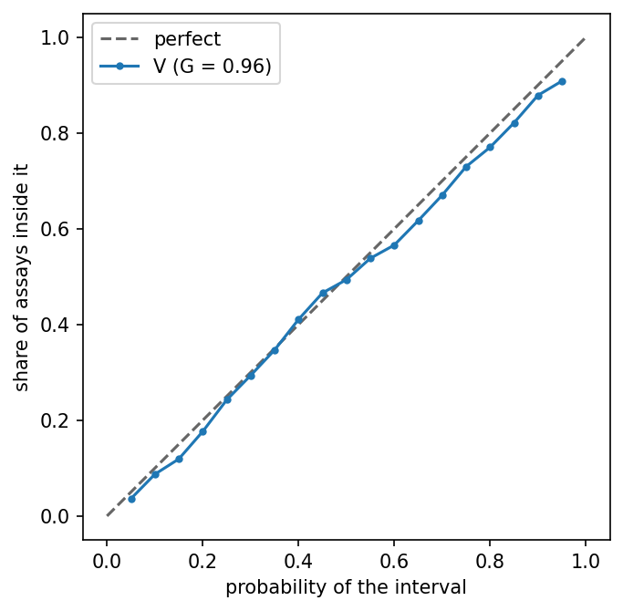
Below the 1:1 line the intervals are too narrow for the errors they have
to cover, and above it the model is hedging. goodness is that departure
summed into one number, and it is the same number the score table
reported.
There is a ready-made accuracy() figure on the plotting objects, and it
is the one to use on a genuine validation set (chapter 14 does). It asks
the model for measurement intervals at the container’s own locations,
which on oof would let the full model interpolate its own training data
and flatter itself. The PIT version above avoids that, because the
distributions it summarizes came from the fold models.
Two more figures read the container alone:
explore = geoml.plots.Explorer(oof, continuous="V")

figure = explore.spread_check(bins=6)
figure.savefig("figures/13-spread-check.png", dpi=150,
               bbox_inches="tight")
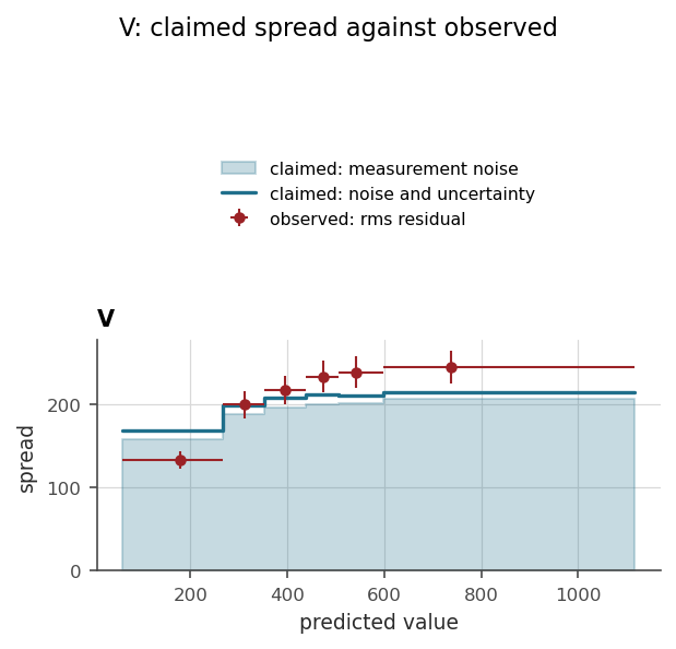
spread_check compares the spread the model claimed against the spread
the errors actually had, laid out along the predicted value, and the level
axis says which term is at fault. A shortfall that widens with the grade
points at the noise model, and a flat one at the posterior. Here the claim
and the errors agree in every bin, within the error bars.
figure = explore.variogram(n_lags=12)
figure.savefig("figures/13-variogram-fan.png", dpi=150,
               bbox_inches="tight")

figure = explore.variogram(n_lags=12, residuals=True)
figure.savefig("figures/13-variogram-residuals.png", dpi=150,
               bbox_inches="tight")
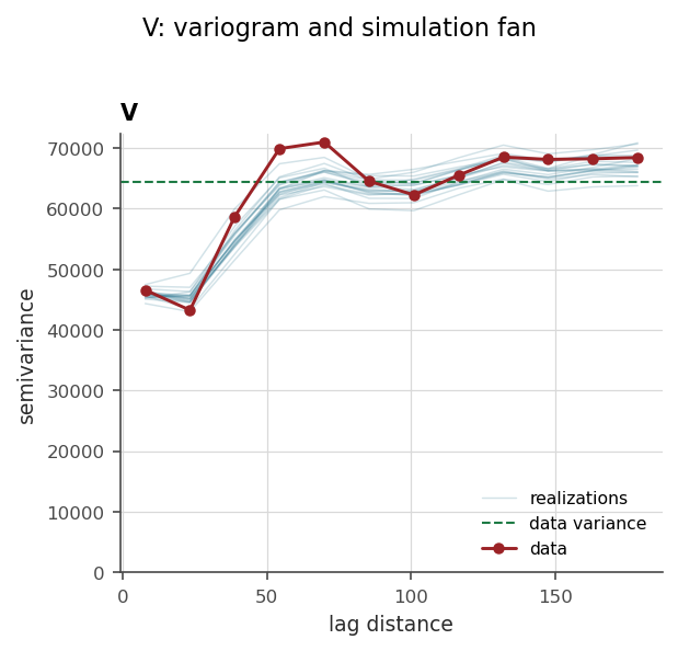
The variogram figure draws the data’s experimental variogram against one
thin curve per simulated realization, computed on the same pairs. Two
corrections happen before the comparison is made, and both matter enough
that without them the figure would libel every model it was shown.
The noise. The measurements carry the likelihood noise, while the
realizations are of the ground with that noise integrated out (chapter 4),
so the two are not the same quantity. An error of its own at each location
adds \((\sigma_i^2 + \sigma_j^2)/2\) to every pair’s contribution, and the
fan is raised by exactly that, read off the noise_variance column. Only
the variance enters, never the shape, so nothing is drawn and the figure
carries no seed.
The clustering. This one is the deeper trap, and it is not about the model at all. Samples follow the ore. An experimental variogram computed on raw pairs therefore describes the sampling as much as the field, and on Walker Lake, whose exhaustive truth is bundled with the package, the raw sample curve runs 1.4 times the true variogram at the sill and 2.3 times at the shortest lag. A model reproducing the field perfectly would look badly over-smooth against it. So each pair is weighted by \(w_i w_j\) from cell-declustering weights, and the sill with it. On Walker Lake that pulls the average departure from the true variogram from 56% down to 12%, and the sill from 89 700 to 64 400 against a truth of 61 800.
Only now can the two curves be laid against each other, and the answer is that this model passes. The fan follows the data’s shape across the whole range, rising where it rises and levelling where it levels, and holds the data inside it at eight lags of the twelve. The data run 2 000 to 4 000 above it between 40 and 70 units, where their curve overshoots its own sill, and below it at the shortest lag, which the caution below is about. The realizations walk like the data.
That verdict is worth pausing on, because it is the opposite of what the same figure said before the two corrections were applied. Uncorrected, the fan sat at a sixth of the data’s curve at short lags and the model looked badly over-smooth. Neither error was in the model. One was a comparison between the ground and a measurement; the other was a comparison against the sampling rather than the field. A diagnostic figure that is not scrupulous about what it puts on each axis will convict an innocent model, and it will do so with an air of authority, because a fan far below a curve looks like evidence.
Scrupulous, it convicts a guilty one too, and this model was one until its Box-Cox was shifted. With the default shift of a millionth, the same figure put the data under the fan’s lowest realization at ten lags of the twelve: by more than 20 000 at the shortest, and the fan about a sixth above the data at long range. The model’s variance was too big, and the noise was the larger part of it. Declustered, the fitted noise alone came to 0.63 of the data’s variance, and noise and ground together to 1.19 of it. The spread check said the same from its own side, claiming a noise of 330 in the highest grades where the errors had 254.
The cause was 22 zero samples. A zero shifted by a millionth has a logarithm far below the rest of the data, and the zeros alone pulled the exponent’s starting value from 0.60 to 0.375; training ended at 0.42. The inverse bent harder with it, and a noise that is constant in the warped space comes back widest where the grade is high, which is where the shortest pairs sit. Shifted by one, the order of the smallest positive value (2.1), the zeros sit beside the rest of the data and the exponent trains to 0.58. The noise falls to 0.48 of the data’s variance, noise and ground together to 0.98, and the fan comes down onto the data. The held-out scores moved with it, rmse from 213 to 212 and CRPS from 122 to 119. Goodness went the other way, from 0.96 to 0.93: the intervals, a little wide before, are now a little narrow, and §13.4 is the patch for that. Where the data hold zeros, the shift wants the size of their smallest positive value, not the default.
One caution remains, and it is the reason the shortest lag is the least trustworthy point here rather than the most damning. Declustering cannot fully mend that bin: the closest pairs exist mainly inside the clusters, so it is built from crowded, high-value ground however the weights are set. On this dataset that can be checked, because Walker Lake ships its exhaustive field. The true variogram reads 26 900 at the shortest lag, and the declustered data read 46 600 there, 1.7 times the truth. That is a limit of the data, and no weighting recovers it. Predicted over the exhaustive grid, the model’s fan follows the true variogram within 7% from the second lag on. At the shortest it sits a third above, because the fitted noise alone, 29 300, is more than the true field varies over 8 units. What the model still gets too high is its nugget, by a little.
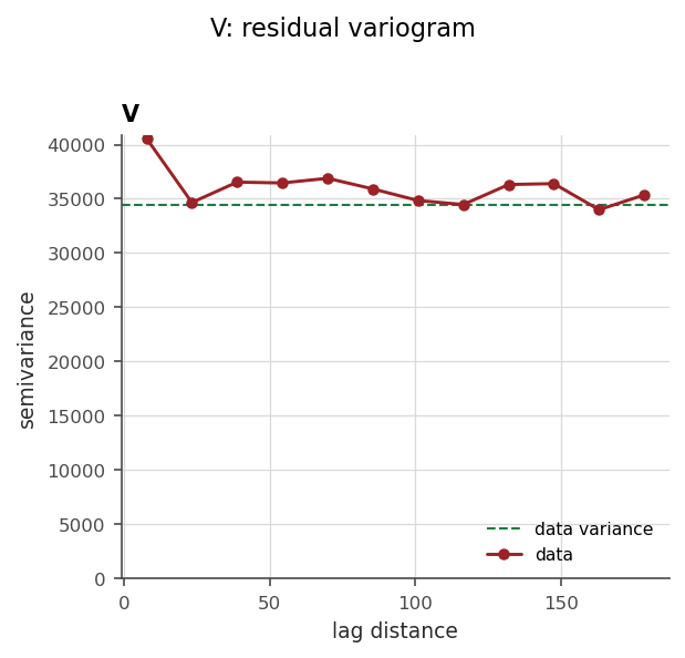
The residual version asks the question no per-location score can: is there
spatial structure left in measured - predicted? Structure in the
residuals is structure the model missed, whether a range fitted too short,
an anisotropy overlooked, or a trend unmodelled. On the out-of-fold
container it is honest by construction.
Here it is flat at its sill from the second lag on, with only the shortest bin riding high — the same crowded, high-value bin the caution above named as the least trustworthy point in either figure. Flat at the sill is what “nothing left” looks like: the residuals are noise with no spatial organization worth naming. That agrees with the fan above, and the two agreeing is worth more than either alone, because they fail in different ways. The fan would miss a model that got the structure right and the level wrong; the residual variogram would miss one whose realizations were individually too smooth while the mean was right.
One more figure, and it is the one that localizes a bias where every score so far aggregated it away. A model can be unbiased over the whole deposit and still run high in the north and low in the south, and only a mean per slab shows where it drifts. That is the swath plot, and the package’s version carries the two corrections without which it describes the drilling rather than the deposit.
walker.decluster(on="V")
model.predict(walker_grid, n_sim=20)
walker_grid.assign_from_data(walker, distance=15.0, hull=40.0)

figure = geoml.plots.Explorer(walker, continuous="V").swath(
    walker_grid, axis="Y", bins=12, where="near_data")
figure.savefig("figures/13-swath.png", dpi=150, bbox_inches="tight")
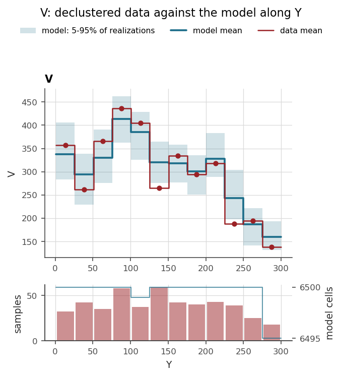
The first correction is the one §13.3 already made for the variogram: the
data’s slab means are declustered, through the column decluster()
stores, so a crowded patch of samples speaks once rather than twenty
times. The second is new, and it is the part a swath plot usually gets
wrong. The model’s slab means run over the grid, and a grid holds ground
the samples never spoke for – air, waste, the far corners of the box –
where the model is extrapolating and its mean says nothing a sample could
be compared with. assign_from_data names the ground the data informs:
within a distance of a sample, inside the data’s concave hull at a chosen
length, or both. The hull is what makes it honest on drilling: it fills
the interior between fences closer than its length, where a ball around
each hole would leave a gap, and leaves out a notch wider than that, where
a convex hull would bridge across. On a drillhole dataset the lengths go
through a transform – an Anisotropy3D with the ranges of the drilling,
dense down the hole and sparse across – so that “near” means what the
geometry means by it. Walker Lake’s samples cover the whole area, so here
the column changes little; on a block model built around a deposit it is
the difference between a swath and a lie.
The band is what a kriging swath cannot draw: each realization’s slab mean taken separately, and the two quantiles between them. The data’s mean sitting inside it, slab after slab, is the model saying it did not know better – outside it, the model saying it did.
13.4 Holding the intervals to their word
The scores may now say the intervals are miscalibrated, with a goodness
well below one and coverage that misses its nominal level. Refitting the
model is the real cure. Conformal calibration is the honest patch, and it
comes with a guarantee. It is built on the same PIT columns the accuracy
plot above used, mapped into one monotone correction:
calibration = geoml.models.conformalize(oof, "V")
print(round(calibration.nominal(0.9), 3))
nominal(0.9) answers a practical question: at what level must a central
interval be cut so that it actually covers 90% of fresh measurements?
For a calibrated model the answer is 0.9 and nothing changes. Above it,
the model claimed more precision than it delivered, and the returned level
is exactly how much wider to cut. The finite-sample guarantee of split
conformal prediction rides on the folds, since exchangeability fails point
by point on spatial data, and folds that mimic deployment (§13.1) are what
makes the out-of-fold PITs stand for the prediction task.
Applying it takes measurement samples at new locations:
new_points = geoml.data.PointData.from_array(
    np.asarray(walker_grid.coordinates)[::100])

samples = model.predict_measurements(new_points, n_sim=20)["V"]
lower, upper = calibration.interval(samples[:, 0, :], coverage=0.9)

print(lower.shape, round(float(np.mean(upper - lower)), 1))
Three limits, stated rather than discovered.
The intervals are of measurements. The ground is never observed, so there is nothing to calibrate a ground interval against.
The guarantee is worth as much as the folds resemble deployment, which is why the calibration and the fold builder are one pipeline rather than two features.
The repair is bounded by the ensemble’s own range.
nominal(q) == 1.0is a warning that the model was too sure for its own samples to say how much wider the interval must be. Raisen_sim, or fix the model rather than the interval.
In the code.
PointData.spatial_k_foldbuilds the folds,models.cross_validate(..., refit=, method=, iterations=, epochs=)drives the loop and returns the out-of-fold container and the score table, andmodels.conformalizereads the PIT metadata. The scores live ingeoml.metricsand are also reported by every continuous variable’scompute_metrics(). Design record with the refit measurements:docs/cross-validation.md.
Further reading
Linnenbrink et al. (2024) for nearest-neighbour distance matching; Roberts et al. (2017) and Wadoux et al. (2021) for the two failure modes the matching resolves; Deutsch (1997) for the accuracy plot; Gneiting & Raftery (2007) for proper scoring rules and Scheuerer & Hamill (2015) for the variogram score; Vovk et al. (2005) and Angelopoulos & Bates (2023) for conformal prediction.
References
Angelopoulos, A. N., & Bates, S. (2023). Conformal prediction: a gentle introduction. Foundations and Trends in Machine Learning, 16(4), 494–591.
Deutsch, C. V. (1997). Direct assessment of local accuracy and precision. In E. Y. Baafi & N. A. Schofield (Eds.), Geostatistics Wollongong ‘96 (pp. 115–125). Kluwer.
Gneiting, T., & Raftery, A. E. (2007). Strictly proper scoring rules, prediction, and estimation. Journal of the American Statistical Association, 102(477), 359–378.
Linnenbrink, J., Milà, C., Ludwig, M., & Meyer, H. (2024). kNNDM CV: k-fold nearest-neighbour distance matching cross-validation for map accuracy estimation. Geoscientific Model Development, 17, 5897–5912.
Rasmussen, C. E., & Williams, C. K. I. (2006). Gaussian Processes for Machine Learning. MIT Press.
Roberts, D. R., Bahn, V., Ciuti, S., Boyce, M. S., Elith, J., Guillera-Arroita, G., … Dormann, C. F. (2017). Cross-validation strategies for data with temporal, spatial, hierarchical, or phylogenetic structure. Ecography, 40(8), 913–929.
Scheuerer, M., & Hamill, T. M. (2015). Variogram-based proper scoring rules for probabilistic forecasts of multivariate quantities. Monthly Weather Review, 143(4), 1321–1334.
Vovk, V., Gammerman, A., & Shafer, G. (2005). Algorithmic Learning in a Random World. Springer.
Wadoux, A. M. J.-C., Heuvelink, G. B. M., de Bruin, S., & Brus, D. J. (2021). Spatial cross-validation is not the right way to evaluate map accuracy. Ecological Modelling, 457, 109692.