17. Case study: a folded quartz vein
The last case study is the one the first two could not be: a real orebody
in three dimensions, logged in drillholes, where the deliverable is a
surface rather than a map. Fifty-three holes intersect a thin quartz
vein folded through the host rock. Two categories, Vein and Waste, and
one question: where is the contact, and how sure are we?
This is also the chapter where a stationary model is visibly not enough, which makes it the natural home for the deep network of chapter 5. Both models are built and both surfaces are drawn, so the cost and the gain are on the same page.
The data is fetched from the public copies used by the tutorial notebooks, about 20 kB in total, and cached beside the chapter, so only the first run needs a connection.
17.1 The database
import io
import os
import urllib.request

import numpy as np
import pandas as pd
import matplotlib.pyplot as plt

import geoml

os.makedirs("figures", exist_ok=True)
os.makedirs("data", exist_ok=True)
geoml.set_seed(1234)

BASE = "https://drive.google.com/uc?export=download&id="
SHEETS = {"vein-collar.csv": "1AT-Hp540CzBP6UFDt6X7MwNTgQ0NA8Gs",
          "vein-lito.csv": "1ktNiQmvsETtIlXu1fhHFW3jzHRFI0BvW"}

for name, key in SHEETS.items():
    local = os.path.join("data", name)
    if not os.path.exists(local):
        raw = urllib.request.urlopen(BASE + key, timeout=60).read()
        pd.read_excel(io.BytesIO(raw)).to_csv(local, index=False)

collar = pd.read_csv("data/vein-collar.csv")

# the log also carries per-interval coordinates; they are not variables,
# and geoML computes them from the collar and survey anyway (chapter 9)
lito = pd.read_csv("data/vein-lito.csv",
                   usecols=["HOLE", "FROM", "TO", "SIMPLE LITO"])

holes = geoml.data.DrillholeData(
    collar,
    hole="HOLE", x="EAST", y="NORTH", z="RL", length="TDEPTH")

holes.add_intervals("lito", lito,
                    hole="HOLE", fr="FROM", to="TO",
                    categorical=["SIMPLE LITO"])

print(holes)
Fifty-three vertical holes and about 5.6 km drilled: a small database by any standard, and the point of the chapter is that the geometry, not the sample count, is what makes it hard.
Note what the summary reports: 247 intervals from a file with 250
rows. The three missing ones belong to a hole, GL76, that the
lithology log records and the collar file does not, so there is nowhere to
put them in space. add_intervals warns and drops them rather than
guessing a collar, which is the behaviour to want. A silent guess here
would place three intervals at a fabricated location, and every model
downstream would honour them. Real databases disagree with themselves at
the edges, and the useful thing a tool can do is say where. Pass
on_error="raise" to make it a hard stop instead, which is the right
setting in a pipeline that should never proceed on a partial database.
17.2 From logged intervals to contacts
Chapter 9’s conversion applies, with one preparatory step. The log records
many touching intervals of the same rock, and the contacts are what carry
information about the surface. merge_domains collapses each run of one
category into a single interval, so that the conversion drops points along
genuine runs and puts a contact only where the rock actually changes.
merged = holes.merge_domains(("lito", "SIMPLE LITO"))
holes.add_intervals("lito", merged)

# two conversions from the same logs, at two spacings
dense = holes.as_classification_input(("lito", "SIMPLE LITO"), length=1.0)
sparse = holes.as_classification_input(("lito", "SIMPLE LITO"), length=10.0)

print(dense.tree())
print(dense.n_data, "training points,",
      sparse.n_data, "inducing points")
print("contacts:", int(np.sum(dense.values("SIMPLE LITO/boundary"))))
The dense conversion is what the model is trained on, and the sparse one is where the inducing points go. That is chapter 3’s separation made concrete: the inducing set summarizes the region, and there is no reason for it to be as dense as the data.
coordinates = np.asarray(dense.coordinates)
rock = dense.values("SIMPLE LITO/measurements_a")

figure = plt.figure(figsize=(7.5, 6))
axes = figure.add_subplot(projection="3d")

for name, colour, size in [("Waste", "0.8", 1), ("Vein", "goldenrod", 6)]:
    mask = rock == name
    axes.scatter(coordinates[mask, 0], coordinates[mask, 1],
                 coordinates[mask, 2], s=size, c=colour, label=name,
                 depthshade=False)

axes.legend(loc="upper left")
axes.set_xlabel("East")
axes.set_ylabel("North")
axes.set_zlabel("RL")
axes.view_init(elev=28, azim=-120)

figure.savefig("figures/17-vein-holes.png", dpi=150, bbox_inches="tight")
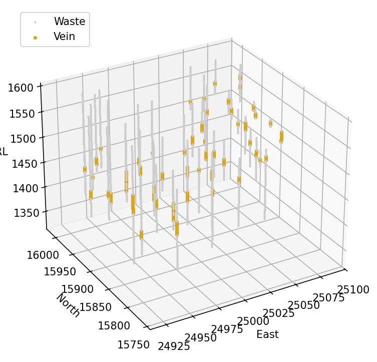
The vein intersections trace a surface that dips and rolls: a shape a single anisotropy ellipsoid can approximate but not follow.
17.3 The stationary baseline
The model of chapter 6, in 3D. One latent field, turned into two category
indicators by a Linear node, with an ellipsoid initialized from a look
at the data and free to move during training. Both models in this chapter
share that construction, so it is worth naming once. The stationary one
trains on the whole dataset at every step, a thousand of them.
def implicit_model(root_node, data, isotropic=False):
    """A one-field implicit model on the given input node."""
    field = geoml.latent.BasicGP(root_node, size=1, isotropic=isotropic)
    indicators = geoml.latent.Linear(field, size=2)

    return geoml.models.VGPNetwork(
        data, "SIMPLE LITO",
        geoml.likelihood.CategoricalGaussianIndicator(2),
        indicators,
        options=geoml.models.GPOptions(jitter=1e-6, training_batch_size=500,
                                       verbose=False))


flat_input = geoml.latent.BasicInput(
    inducing_points=sparse,
    transform=geoml.transform.Anisotropy3D(
        100, 1.0, 0.5, azimuth=270, dip=45),
    center=True)

flat_model = implicit_model(flat_input, dense)
flat_model.set_learning_rate(2e-2)
flat_model.train_full(max_iter=1000)
17.4 The deep model: moving the ground before modelling it
Chapter 5’s argument, applied. Rather than asking one ellipsoid to
describe a folded surface, let a vector field move the coordinates and
model a stationary field in the moved space. GPWalk integrates the
movement in a few steps, and everything downstream is unchanged: the same
one-field implicit model, reading transformed coordinates – with one range
instead of three. The ellipsoid still carries the anisotropy the model
starts from; the walk bends the space from there, and a range per
direction in the field reading it would be a second way to say the same
thing, which training resolves into a stretched, overconfident field.
The deep model trains differently. It has more local optima than the
stationary one, so it trains on minibatches of 500 rows (chapter 11’s
train_svi), whose noise helps it out of a poor start: twenty epochs at a
high learning rate to find the shape, then sixty at a lower one to settle
it. set_learning_rate restarts the optimizer, which is the point of
calling it between the two. Where it starts still matters: built after the
stationary model has drawn from the random stream, it settled on a
fragmented vein, so it gets the chapter’s seed again, which the figures
below were drawn from. Trying a few seeds and keeping the one with the
best held-out score (chapter 13) is the honest way to choose.
geoml.set_seed(1234)

deep_input = geoml.latent.BasicInput(
    inducing_points=sparse,
    transform=geoml.transform.Anisotropy3D(
        100, 1.0, 0.5, azimuth=270, dip=45),
    center=True)

displacement = geoml.latent.BasicGP(deep_input, size=3)
walked = geoml.latent.GPWalk(displacement, n_steps=5)

deep_model = implicit_model(walked, dense, isotropic=True)
deep_model.set_learning_rate(5e-2)
deep_model.train_svi(20)
deep_model.set_learning_rate(1e-2)
deep_model.train_svi(60)

figure, axes = plt.subplots(figsize=(7, 4.2))
axes.plot(flat_model.training_log, label="stationary (iterations)")
axes.plot(deep_model.training_log, label="deep (GPWalk, minibatches)")
axes.set_xlabel("step")
axes.set_ylabel("ELBO")
axes.legend()

figure.savefig("figures/17-elbo.png", dpi=150, bbox_inches="tight")
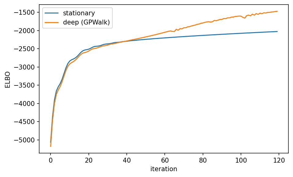
The stationary model ends at the higher bound, and that is not the verdict it looks like. A bound rewards fitting the training points, and a thousand full steps on one ellipsoid buy that hole by hole; the deep model’s bound is a minibatch estimate, noisier and lower, and it spends part of what it has on a vector field. Which vein is the better one is a question about the ground between the holes, which neither bound sees – the surfaces below are the first look at it, and chapter 13’s held-out check the honest one.
17.5 The surfaces
The deliverable is the zero level set of the vein’s indicator. Contour it
out of a block model, then predict onto the resulting surface so that
every triangle carries the model’s uncertainty there. The blocks start at
20 m and refine (chapter 8) cuts them down to 2.5 m wherever the
vein’s boundary runs through them, so the resolution goes to the contact
and nowhere else. A regular grid at 2.5 m would hold two million points
for the same surface, and a coarser one draws a walked surface in steps:
the walk folds the space, which puts sharper features on the lattice than
a stationary field does. Both models get the same treatment.
surfaces = {}

for name, trained in [("stationary", flat_model), ("deep", deep_model)]:
    blocks = geoml.data.BlockSet3D(
        start=[24860, 15710, 1310],
        n=[15, 18, 15],
        step=[20.0, 20.0, 20.0],
        discretization=(2, 2, 2),
        max_levels=3)
    blocks = geoml.models.refine(trained, blocks)
    surface = blocks.get_contour("SIMPLE LITO/Vein/indicator_predicted", 0.0)
    trained.predict(surface)
    surfaces[name] = surface
    print("%-11s %6d blocks, %6d triangles, %8.0f m2"
          % (name, blocks.n_data, len(surface.triangles), surface.area))
The contour is taken at zero because the category indicators are log-odds.
The surface where Vein stops losing to Waste is the contact, and
chapter 6’s ind_skew is the same quantity read as a cut-off. Predicting
onto the surface is the second call: a mesh is a spatial object like any
other, so it takes a prediction, and what it carries is the model’s
uncertainty about the very boundary it draws.
figure = plt.figure(figsize=(13, 5.6))

for position, name in enumerate(["stationary", "deep"], start=1):
    surface = surfaces[name]
    vertices = np.asarray(surface.coordinates)
    uncertainty = surface.values("SIMPLE LITO/uncertainty")

    axes = figure.add_subplot(1, 2, position, projection="3d")
    drawn = axes.plot_trisurf(
        vertices[:, 0], vertices[:, 1], vertices[:, 2],
        triangles=surface.triangles, cmap="cividis", linewidth=0,
        antialiased=False)

    # colour by uncertainty rather than by elevation, which is what
    # plot_trisurf would use if left to itself
    drawn.set_array(uncertainty[surface.triangles].mean(axis=1))
    drawn.set_clim(0.0, 1.0)

    figure.colorbar(drawn, ax=axes, shrink=0.55, label="uncertainty")
    axes.set_title(name)
    axes.set_xlabel("East")
    axes.set_ylabel("North")
    axes.set_zlabel("RL")
    axes.set_zlim(1300, 1600)
    axes.view_init(elev=34, azim=-118)

figure.savefig("figures/17-vein-surface.png", dpi=150,
               bbox_inches="tight")
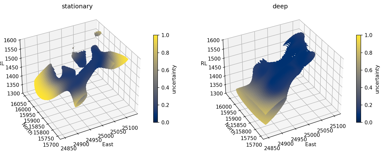
The colour is the part a CAD-drawn wireframe cannot carry. Both surfaces are dark where holes constrain them and pale where they do not, which is the map of where the next hole is worth drilling.
The difference between the two is the fold. One ellipsoid has to describe a surface whose attitude changes along strike, and it cannot: the stationary answer breaks into pieces, loses the vein between hole fences, and flares into high-uncertainty skirts at the edges of the model. The walked input lets the same kernel follow the roll, and the deep answer is a single coherent sheet that stays with the intersections and only opens up past the last hole. The uncertainty colouring is what makes the comparison fair, because it distinguishes a surface the model is committing to from one it is guessing at.
17.6 Where the walk moved the ground
The deep model’s answer rests on a node nobody measured: walked, the
coordinates after the walk. predict_node stops the model’s prediction at
any node of the tree and writes what that node says into a container, as
predict writes what the leaves say. Here it is asked where the walk takes
every point of a plan section through the vein, and the answer is set
against where the input put them before the walk.
section = geoml.data.Grid3D(start=[24850, 15700, 1450], n=[31, 36, 1],
                            step=[10, 10, 10])
moved = deep_model.predict_node(walked, section, labels=["u", "v", "w"])

# where the input puts the same points: its transform, about its centre
deep_input.transform.refresh()
before = np.asarray(deep_input.transform(
    np.asarray(section.coordinates) - deep_input.center))
shift = moved.get_predictions() - before
print("the walk moves a point by %.2f ranges at most, %.2f on average"
      % (np.linalg.norm(shift, axis=1).max(),
         np.linalg.norm(shift, axis=1).mean()))

plan = np.asarray(section.coordinates)
figure, axes = plt.subplots(figsize=(6.5, 6.5))
arrows = axes.quiver(plan[:, 0], plan[:, 1], shift[:, 0], shift[:, 1],
                     np.linalg.norm(shift, axis=1), cmap="viridis")
figure.colorbar(arrows, ax=axes, shrink=0.7,
                label="displacement, in ranges")
axes.set_aspect("equal")
axes.set_xlabel("East")
axes.set_ylabel("North")
axes.set_title("The walk at RL 1450, in the transformed space")

figure.savefig("figures/17-walk.png", dpi=150, bbox_inches="tight")
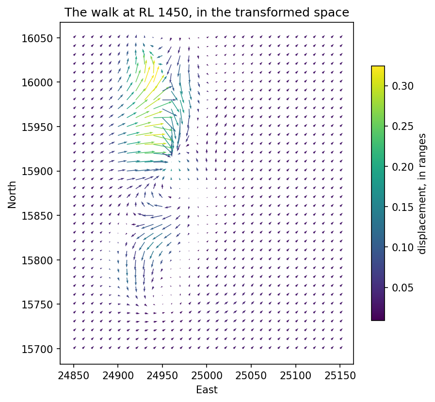
The arrows live in the space the input’s ellipsoid made, where one unit is one range, so they say how far the walk carries each point measured in the lengths the stationary field sees. Where they are short the walk leaves the ground alone and the ellipsoid alone describes it; where they swing, the walk is doing the folding.
moved is a LatentVariable: one part per output of the node, each
holding the node’s latent_mean and latent_variance and its
realizations, all on the latent scale, since a node has no likelihood to
back-transform through. It is saved, subsetted and read by path like any
other variable, under the node’s own name unless name= gives another
(section.values(moved.name + "/u/latent_mean") is the first
coordinate). A node is predicted at points only; a block’s value is
an average a likelihood takes, and a node has none.
17.7 Did the fold help?
A surface that fits better is not automatically a better model. The comparison that counts is on samples the model did not see, and with 53 holes the split that respects the geometry is by hole (chapter 13).
flat_model.predict(dense)
flat_predicted = dense.values("SIMPLE LITO/predicted").copy()

deep_model.predict(dense)
deep_predicted = dense.values("SIMPLE LITO/predicted").copy()

interior = ~dense.values("SIMPLE LITO/boundary").astype(bool)
truth = dense.values("SIMPLE LITO/measurements_a")

for name, predicted in [("stationary", flat_predicted),
                        ("deep      ", deep_predicted)]:
    agree = np.mean(predicted[interior] == truth[interior])
    print("%s in-sample agreement: %.3f" % (name, agree))
These are in-sample numbers, printed with that label because the point of
chapter 13 is that in-sample numbers flatter every model. Here they flatter
the stationary one: it agrees with every training point and draws the vein
as tubes along the holes, where the deep model gives up a few points and
draws one sheet between them. A model can memorize 53 holes in more than
one way, so the honest comparison runs cross_validate with the folds cut
on HOLEID, which every conversion in chapter 9 carried as metadata
precisely for this. The numbers above illustrate the machinery rather than
settle the geology.
In the code.
geoml.latent.GPWalkis the SDE node, andgeoml.transform.Anisotropy3Dthe ellipsoid it takes the burden off.VGPNetwork.predict_nodewrites any node’s prediction as ageoml.data.LatentVariable.models.refinecuts adata.BlockSet3Dwhere the contact runs andBlockSet3D.get_contour(path, value)builds the surface; meshes take predictions like any container, andMesh3D.simplify,.smoothand the booleans of chapter 12 apply to the result.DrillholeData.merge_domainscollapses the runs the log records, andas_classification_inputputs the contacts in at zero support.
Further reading
The potential-field formulation is Lajaunie et al. (1997), geoML’s machine-learning reading of it is the 2017 paper, and the categorical treatment used here is the 2023 one. The deep model and this dataset are the subject of the 2025 paper, where the fold is examined properly rather than at a manual’s iteration counts.
References
Gonçalves, Í. G. et al. (2017). A machine learning approach to the potential-field method for implicit modeling of geological structures. Computers & Geosciences.
Gonçalves, Í. G. et al. (2023). Variational Gaussian processes for implicit geological modeling. Computers & Geosciences. https://linkinghub.elsevier.com/retrieve/pii/S0098300423000274
Gonçalves, Í. G. et al. (2025). Uncertainty propagation in deep Gaussian process networks. Mathematical Geosciences. https://doi.org/10.1007/s11004-025-10187-4
Lajaunie, C., Courrioux, G., & Manuel, L. (1997). Foliation fields and 3D cartography in geology: principles of a method based on potential interpolation. Mathematical Geology, 29(4), 571–584.