10. Containers and addressing

Everything a model reads or writes lives in a container: PointData for scattered samples, Grid1D/Grid2D/Grid3D for regular lattices, BlockSet3D for the refinable block model of chapter 8, plus the directional and mesh types the later chapters use. They differ in how they hold coordinates and agree on everything else, and this chapter is about that shared part: how to find a number, how to get it out, and how to move a container between scripts.

10.1 One tree, addressed by path

A container is a tree of variables, their components, their attributes and per-location metadata. Every leaf has a path, and the path is the one true name: the same spelling in memory, in the Zarr store, and in this manual.

Four verbs cover almost everything.

call	what it gives you
container.tree()	the picture: every variable and every column
container.values(path)	the column as a NumPy array
container.get(path)	the column object, for drawing and contouring
container.select(pattern)	the paths matching a glob

tree() first, always, and especially after a prediction:

import os

import geoml
import numpy as np

os.makedirs("figures", exist_ok=True)
geoml.set_seed(1234)

walker, walker_grid = geoml.datasets.walker()

covariance = geoml.kernels.Covariance(
    kernel=geoml.kernels.Spherical(),
    transform=geoml.transform.Isotropic(100.0))

model = geoml.models.GP(
    data=walker,
    variable="V",
    covariance=covariance,
    warping=geoml.warping.ZScore(1),
    options=geoml.models.GPOptions(verbose=False))

model.train(20)

grid = geoml.data.Grid2D(start=[1, 1], n=[60, 60], step=[4.3, 5.0])
model.predict(grid, n_sim=20)

grid.get("V").reset_quantiles([0.1, 0.5, 0.9])

print(grid.tree())

Everything the model wrote is a leaf in that tree: the prediction, the variances, the realizations and the quantiles. Reading a value is then a matter of spelling its path.

prediction = grid.values("V/prediction")
median = grid.values("V/quantiles/0.5")
spread = grid.values("V/quantiles/0.9") - grid.values("V/quantiles/0.1")

print(prediction.shape, median.shape, spread.shape)
print("mean grade:", round(float(np.mean(prediction)), 1))
print("mean 0.1-0.9 spread:", round(float(np.mean(spread)), 1))

select answers the same question with a glob, which is how a script loops over things it did not name in advance:

print(sorted(str(path) for path in grid.select("V/quantiles/*")))
print(sorted(str(path) for path in grid.select("**/prediction")))

select hands back path objects rather than strings, which is why they are printed through str. Anywhere a path is expected, either form is accepted.

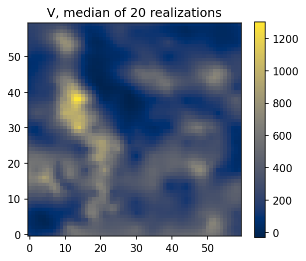
values for what you compute with, get for what you draw. values returns a plain array, decoded if the column stores text as integer codes. get returns the column object, which knows things an array does not: how to reshape itself onto a grid (as_image), how to contour itself into a surface (get_contour), and what its labels are.

import matplotlib.pyplot as plt

image = grid.get("V/quantiles/0.5").as_image()

figure, axes = plt.subplots(figsize=(4.6, 4.4))
drawn = axes.imshow(image, origin="lower", cmap="cividis")
figure.colorbar(drawn, ax=axes, shrink=0.85)
axes.set_title("V, median of 20 realizations")
figure.savefig("figures/10-median.png", dpi=150, bbox_inches="tight")

One trap worth naming once. get(path).values is not an array, it is the storage object behind the column, and converting a large one into an array loads the whole thing into memory. Use values(path) when an array is what you want.

10.2 The paths a model writes

Most of the manual is spent reading these, so here they are in one place. V stands for a continuous variable’s name and <c> for a cut-off.

path	what it holds
V/measurements	what was observed, where anything was
V/prediction	the model’s value for the ground
V/latent_variance	how sure the model is
V/noise_variance	how far a measurement would scatter
V/dispersion	how much the ground varies inside a block
V/simulations/<i>	one realization
V/quantiles/<q>	a quantile of the realizations
V/proportions/<c>	the share above a cut-off, on a block model
V/divided/<c>	how often the realizations disagree about the cut-off

The last two appear only where a block has an interior for the cut-off to cross, so they are written by a BlockSet3D prediction and not by a grid or a point one (chapter 8).

A vector or compositional variable puts its components one level down, so Jura’s zinc is Elements/Zn/prediction. A categorical variable reports Landuse/predicted and Landuse/uncertainty for the whole variable, and Landuse/Forest/probability for a single class. Metadata, the per-location facts of chapter 9, sits under _metadata/:

print(sorted(str(path) for path in walker.select("**"))[:6])

10.3 Getting the numbers out

Three doors, by destination, and one of them is not an export at all.

import tempfile

frame = grid.as_data_frame()
print([name for name in frame.columns if name.startswith("V_")][:5])

path = os.path.join(tempfile.mkdtemp(), "walker-grid.zarr")
grid.to_zarr(path)
back = geoml.data.Grid2D.open(path)

print(type(back).__name__, back.n_data,
      bool(np.allclose(back.values("V/prediction"),
                       grid.values("V/prediction"))))

as_data_frame flattens the paths into column names (V_quantiles_0.5) for spreadsheets and general software. as_pyvista does the same for 3D viewers, with a prettier spelling (V - prediction), and carries the mapping back to real paths alongside the mesh, so nothing has to be parsed out of a name.

to_zarr is the one that is not an export. It writes the entire container, coordinates, every variable’s tree, metadata and simulations included, and open rebuilds it with its type intact. It is lossless and appendable, a reopened container can be predicted into again, and it is the natural hand-off between a modelling script and a reporting one. Model persistence (chapter 11) is a separate mechanism for a separate thing: a model is constructors and parameters, a container is arrays.

10.4 When the ensemble outweighs the machine

A block model’s simulations run to hundreds of gigabytes on real jobs, so containers keep their arrays in a store that is memory-resident when small and chunked on disk when not. Chunks split the location axis only, so a chunk holds whole rows: every realization of a band of blocks. Two habits follow, and they are the only two worth remembering.

Read one realization at a time. A realization has a path of its own, and reading it costs one column of memory whatever the store holds. This is the primitive under the per-realization arithmetic of chapter 7:

first = grid.values("V/simulations/0")
print(first.shape, round(float(first.mean()), 1))

# the same column as a drawable attribute, for as_image or get_contour
drawable = grid.get("V").simulation(0)
print(type(drawable).__name__)

Reduce over locations a band at a time. Everything in the package that summarizes an ensemble (quantiles, cut-off shares, grade–tonnage curves, the figures) walks the store in bands and holds one at a time. Code you write should do the same. The one call to avoid is asking a large simulations store to become a single array, which on a real block model will end the session.

In the code. The tree machinery lives in data/base.py, the containers in data/containers.py and data/grids.py, Zarr persistence in data/io.py, and the store in storage.py. Design record for the addressing: docs/variable-paths.md.

Further reading

docs/variable-paths.md and docs/variable-block-models.md are the design records behind this chapter, and the Zarr documentation covers the store format the persistence rests on.