6. Categories and boundaries

A rock type is not a number, and pretending it is one, which is indicator kriging’s move, buys a workflow at the price of coherence: probabilities that do not sum to one, order relations violated, and no boundary anywhere, just a raster of memberships. This chapter models categories the way the package models everything else, with latent fields, and gets three things out of one construction: coherent probabilities, an uncertainty map, and contacts as genuine surfaces.

6.1 One field per category

Give each of \(C\) categories its own latent field, and let a location belong to the category whose field is highest there. The fields are not observed. What is observed is the winner, a logged interval, and the likelihood turns each observation into the statement “this category’s field beats the others here”, which is information about differences between fields. Class probabilities follow from how confidently each field wins, and they sum to one by construction, because exactly one field wins.

The geological reading is the implicit model: what matters is not any field’s magnitude but where two fields cross. The quantity the package computes per category is its log-odds against its best rival, positive where the category rules and negative where it loses, and the contact is that quantity’s zero level set. A boundary is then a contour like any grade shell, which chapter 12 extracts as a mesh, and it carries model uncertainty like everything else. Where the fields cross at a shallow angle the boundary is soft, and the entropy map says so.

Drillholes contribute two kinds of observation, and the distinction is worth respecting when the data is prepared (chapter 9). Interior points are where a category was logged along an interval. Contacts are where two categories meet at a measurable depth, a zero-support observation that pins the crossing exactly. DrillholeData.get_contacts and as_classification_input produce both, which is the construction of the 2023 implicit-modelling paper.

In the code. geoml.likelihood.CategoricalGaussianIndicator is the likelihood, and the variable side is CategoricalVariable or RockTypeVariable, the latter carrying the two-sided measurements a contact has. Per category you get probability, the indicator columns, and the log-odds (ind_skew) whose zero is the contact. Per variable you get predicted, the winning label, and uncertainty, the normalized entropy. GradientIndicator adds structural data, dip and strike read as derivatives of the fields, through the same door.

6.2 Jura’s land use, mapped with its doubt

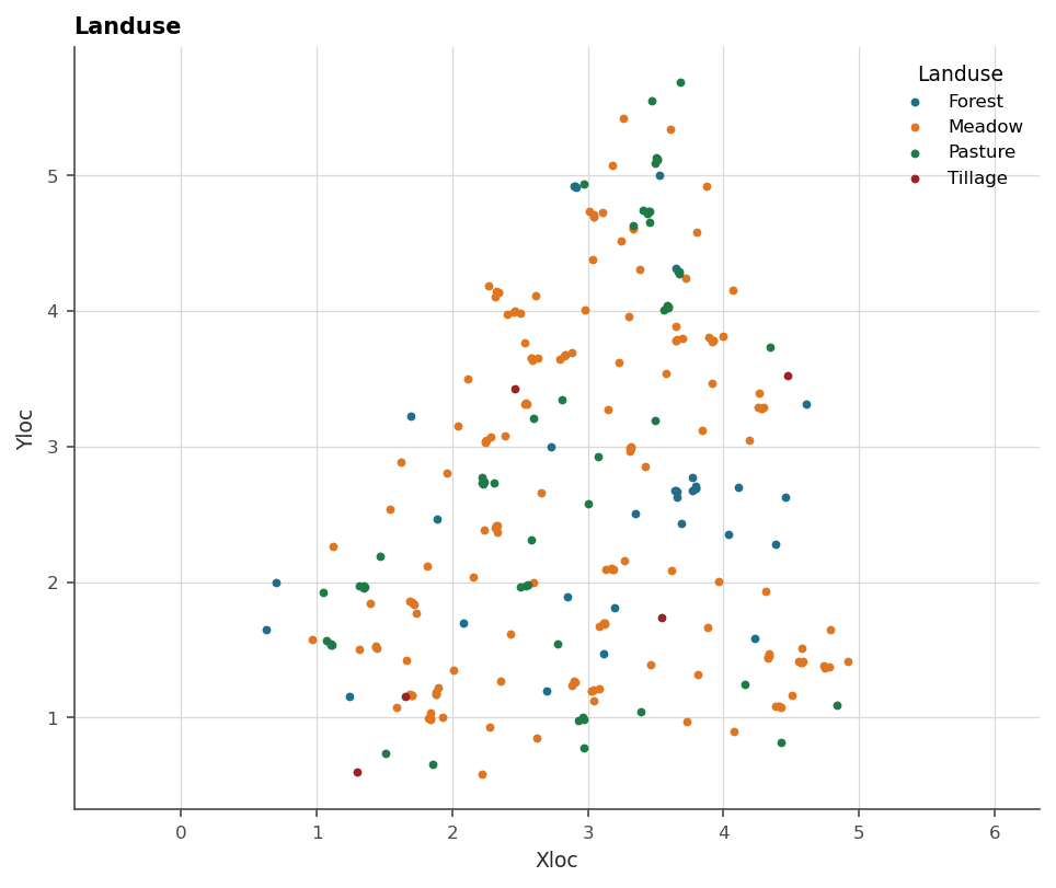
The Jura dataset carries four land-use classes, a rock type and seven heavy metals at 259 sites, with 100 more held out for validation. This chapter uses the land use alone, and chapter 16 comes back for the rest.

import os

import geoml
import numpy as np
import matplotlib.pyplot as plt

os.makedirs("figures", exist_ok=True)
geoml.set_seed(1234)

jura_train, jura_validation = geoml.datasets.jura()
print(jura_train.tree())

labels = list(jura_train.get("Landuse").labels)
print(labels)

The tree shows what a categorical variable holds before anything is predicted: the logged labels in measurements_a and measurements_b, a boundary flag marking contacts, and one child node per category.

figure = geoml.plots.Explorer(jura_train, categorical="Landuse").scene()
figure.savefig("figures/06-jura-landuse.png", dpi=150,
               bbox_inches="tight")

At 259 sites the data itself is a perfectly good inducing set, so the network is as short as it gets. A Matérn kernel keeps the boundaries from being artificially smooth.

root = geoml.latent.BasicInput(
    inducing_points=jura_train,
    transform=geoml.transform.Isotropic(0.5))

gp = geoml.latent.BasicGP(
    root,
    size=len(labels),
    kernel=geoml.kernels.Matern32())

model = geoml.models.VGPNetwork(
    jura_train, "Landuse",
    geoml.likelihood.CategoricalGaussianIndicator(n_components=len(labels)),
    gp,
    options=geoml.models.GPOptions(verbose=False))

model.train_full(max_iter=150)

grid = geoml.data.Grid2D(start=[0, 0], end=[6, 6], n=[201, 201])
model.predict(grid)

The prediction fills the grid with the winning label, the per-category probabilities, and the entropy:

probability = grid.get("Landuse/%s/probability" % labels[0]).as_image()
uncertainty = grid.get("Landuse/uncertainty").as_image()

figure, axes = plt.subplots(1, 2, figsize=(9.5, 4.2), sharey=True)

for ax, image, title in zip(
        axes, [probability, uncertainty],
        ["P(%s)" % labels[0], "uncertainty (entropy)"]):
    drawn = ax.imshow(image, origin="lower", cmap="cividis",
                      extent=(0, 6, 0, 6), vmin=0, vmax=1)
    figure.colorbar(drawn, ax=ax, shrink=0.8)
    ax.set_title(title)

figure.savefig("figures/06-jura-probability.png", dpi=150,
               bbox_inches="tight")

total = sum(grid.values("Landuse/%s/probability" % label)
            for label in labels)
print("probabilities sum to one:", bool(np.allclose(total, 1.0)))

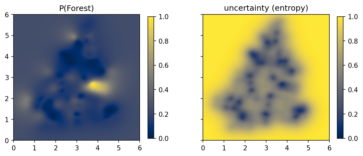
The entropy map is the one to show a geologist first. It saturates everywhere outside the sampled area, where the model has nothing to go on and says so instead of extending the nearest class over the whole square. Inside the sampled area it rises along the boundaries, where the winning field wins narrowly, which is exactly where a mapped contact should be doubted. Chapter 12 turns the log-odds zero into an actual surface for a 3D case, and chapter 17 does it on a real deposit with contacts read from drillholes.

Further reading

The 2023 implicit-modelling paper for the boundary likelihood and the comparison with radial-basis implicit modelling; the 2021 structural-trend paper for dip-and-strike data read as field derivatives; the 2025 paper for categories through deep networks.

References

Gonçalves, Í. G. et al. (2021). A machine learning model for structural trend fields. Computers & Geosciences. https://doi.org/10.1016/j.cageo.2021.104715

Gonçalves, Í. G. et al. (2023). Variational Gaussian processes for implicit geological modeling. Computers & Geosciences. https://linkinghub.elsevier.com/retrieve/pii/S0098300423000274

Gonçalves, Í. G. et al. (2025). Uncertainty propagation in deep Gaussian process networks. Mathematical Geosciences. https://doi.org/10.1007/s11004-025-10187-4

Lajaunie, C., Courrioux, G., & Manuel, L. (1997). Foliation fields and 3D cartography in geology: principles of a method based on potential interpolation. Mathematical Geology, 29(4), 571–584.